Week 1: Channel flow simulation using CONVERGE CFD

SIMULATION OF FLOW INSIDE A CHANNEL USING CONVERGE

AIM: The aim of this project is to simulate the flow in a rectangular duct with dimensions of 0.1m in the X direction and 0.001m in the Y and Z directions using CONVERGE, a CFD solver. The simulation will be set up using the CONVERGE GUI and for solving Linux-based command line operator such as CYGWIN is used for executing the solver stage of simulation. The output results will be analyzed using a post-processing tool such as PARAVIEW, which will be used to render the flow and provide insights into the behavior of the fluid and the properties of the flow.

Intoduction: To understand the differences between CONVERGE and ANSYS, I set up a simulation using CONVERGE to simulate flow in a rectangular duct with a structured mesh. Unlike ANSYS, CONVERGE uses structured meshing exclusively. The simulation setup was straightforward, using the dimensions of 0.1m in the X direction and 0.001m in the Y and Z directions for the duct. After running the simulation, I used PARAVIEW to visualize and analyze the flow. This allowed me to gain insights into the fluid behavior and flow properties using the output results of the simulation.

Why should i use CONVERGE for CFD application?

Converge is a computational fluid dynamics (CFD) software that is used to simulate and analyze fluid flow in complex geometries. Here are some reasons why you might want to use Converge:

1. Accuracy: Converge uses a highly accurate numerical method called the finite volume method, which allows for accurate simulation of fluid flow and heat transfer in complex geometries.

2. Flexibility: Converge is a highly flexible software that can be customized to meet the specific needs of different applications. It allows for customization of boundary conditions, turbulence models, and other parameters, and can be used to simulate a wide range of fluid flow problems, including combustion, sprays, and multiphase flows.

3. Speed: Converge is designed to run efficiently on parallel computing architectures, which means that it can perform simulations quickly and efficiently, even for large and complex geometries.

4. Validation: Converge has been extensively validated against experimental data and other CFD codes, which means that users can have confidence in the accuracy of their simulations.

5. Support: Converge is backed by a team of experienced developers and support staff, who can provide assistance with setup, usage, and troubleshooting.

Overall, Converge is a powerful and versatile CFD software that can be used to simulate and analyze fluid flow in complex geometries with a high degree of accuracy and efficiency. It is a valuable tool for engineers, researchers, and scientists who need to analyze and optimize fluid flow systems.

Why should i use PARAVIEW for CFD application?

Paraview is a powerful scientific visualization software that is widely used in various fields such as engineering, physics, biology, and medicine. Here are some reasons why you might want to use Paraview:

1. Data visualization: Paraview provides a user-friendly interface for visualizing scientific data. It allows you to interactively explore large datasets and gain insights into your data. With Paraview, you can create 2D and 3D visualizations, animations, and streamline visualizations.

2. Data analysis: Paraview provides a wide range of tools for data analysis. You can compute derived quantities, slice and dice data, extract regions of interest, and perform other types of analysis. The software also provides various filters and algorithms for smoothing, interpolating, and resampling data.

3. Collaboration: Paraview is designed to work in a collaborative environment. It allows multiple users to work on the same dataset simultaneously and share their visualizations and analysis with each other.

4. Open-source: Paraview is an open-source software, which means that it is freely available to use and modify. This makes it accessible to a wide range of users, including researchers, students, and educators.

5. Cross-platform: Paraview is available for Windows, macOS, and Linux, making it a versatile software that can be used on different operating systems.

Overall, Paraview is a powerful and versatile tool for scientific data visualization and analysis, and it can help you gain insights into your data and communicate your findings to others.

In CFD setup, the following will be the steps ,

1.Geometry Creation/Pre-Processing

2.Meshing

3.Solving

4.Post-Processing

In this case, the flow of peration is as follows,

1. Creation Of Geometry using CONVERGE
2. Case Setup using CONVERGE (Setting up Material selection,Boundary conditions, Mesh criteria, Initialization Conditions, Solver parameters,Output variables, Writing of Output Files)
3. Exporting Of Input files for solver
4. Calling solver from Input File folder using CYGWIN
5. Writing files using CYGWIN
6. Converting those Output files in Binary format to readable format which contains required output variables.
7. Analysing the output files using PARAVIEW.

Creation Of Geometry using CONVERGE :

In CONVERGE using GEOMETRY tab>CREATE>SHAPE >RECTANGLE 0.1m in the X direction and 0.001m in the Y and Z directions shape has been created. Checked for any Geometrical errors using Diagnosis tool check. Found no errors.

Case Setup :

1.Application Type- Time Based application

• 

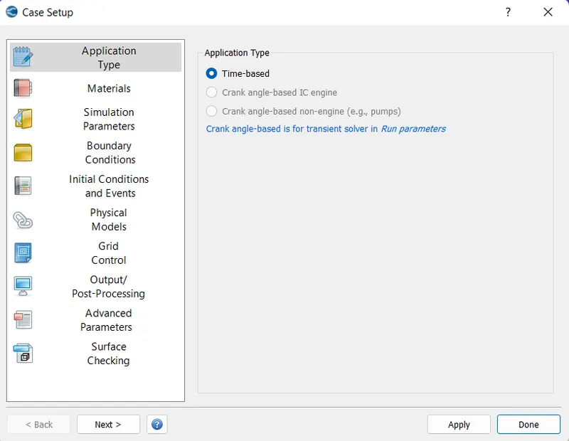
It is choosen as we are going to perform steady state analysis with pressure based flow to be happen from Inlet to Outlet.

2.Materials-

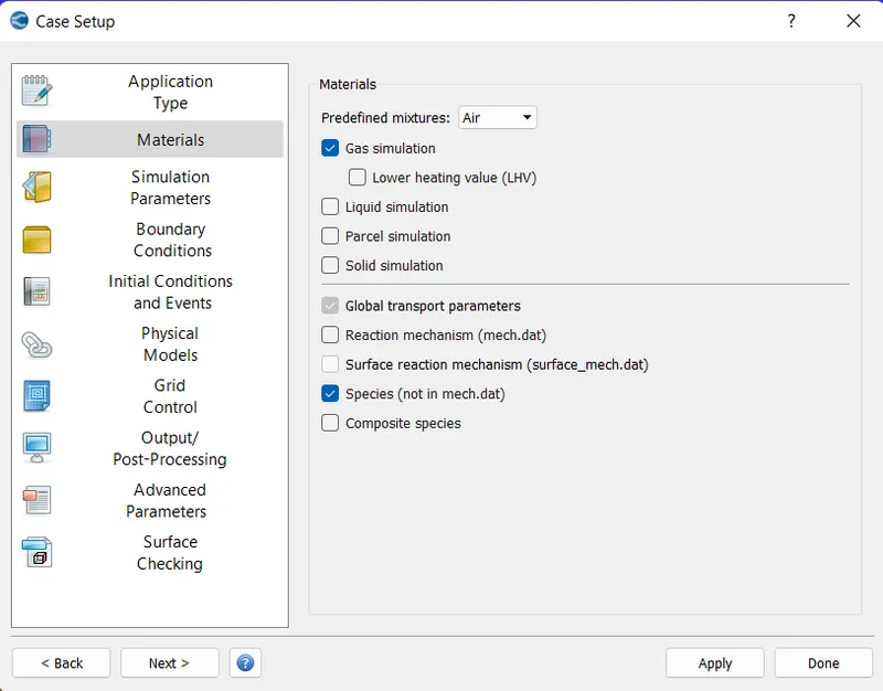
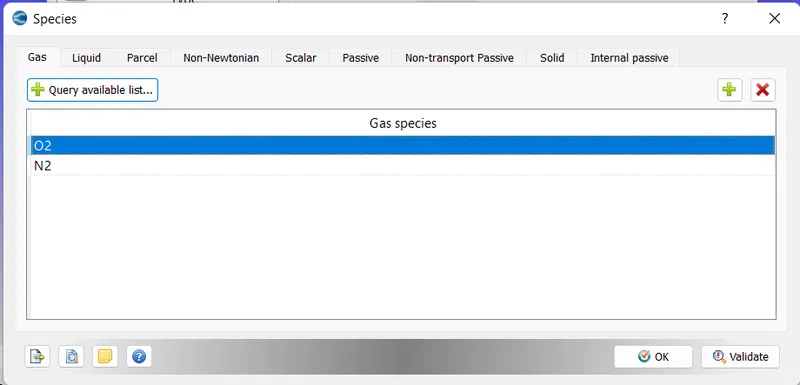
Predefined Mixture AIR has been choosen as working fluid and GAS SIMULATION is enabled. As there is NO chemical reaction is going to take place inside the channel, so the REACTION MECHANISM option is Disabled and in Species option is enabled to specify type of GAS Elements in the Gas Simulation.

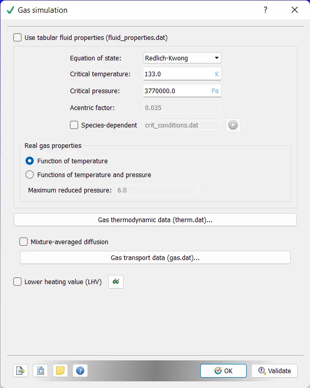
Following were Thermal data of gas present in it and type of Equation used and few other variables of the gas and Type of dependency.

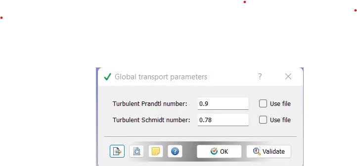
Default Dimensionless numbers has been used. With the help of these numbers we cacn alter the flow behaviour of the fluid.

3.Simulation Parameters:

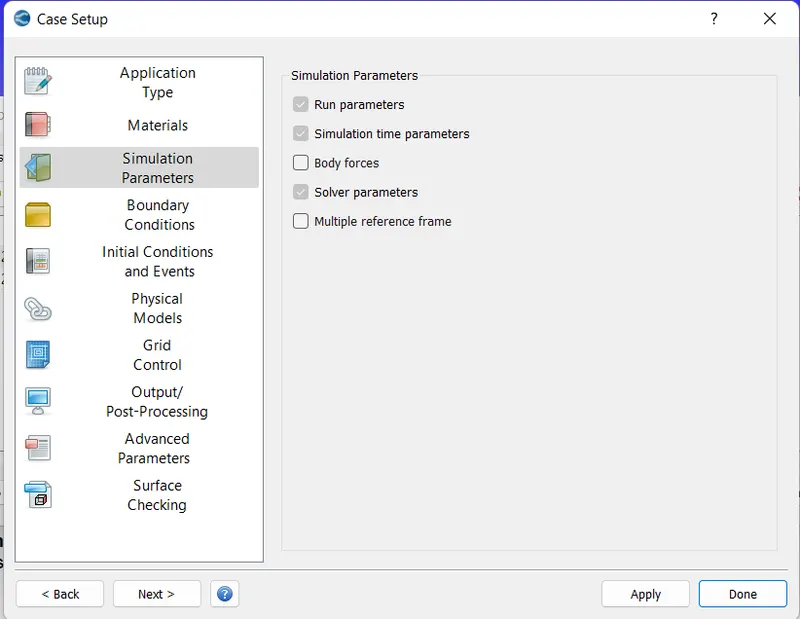
As there is no Body forces acting on the flow like Gravity, disabled the Body forces option. Few options are made default Enable represent that for solving this flow or to simulate this flow it has to be enabled.

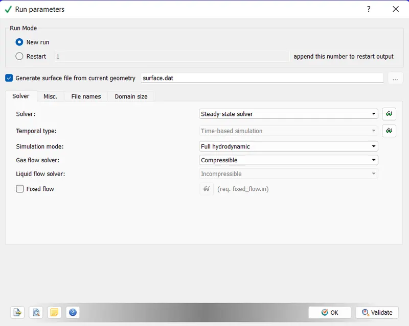
Steady- State Solver is used, Simulation mode of Full Hydrodynamic and Gas Flow solver Compressible is choosen from Run Parameters tab.

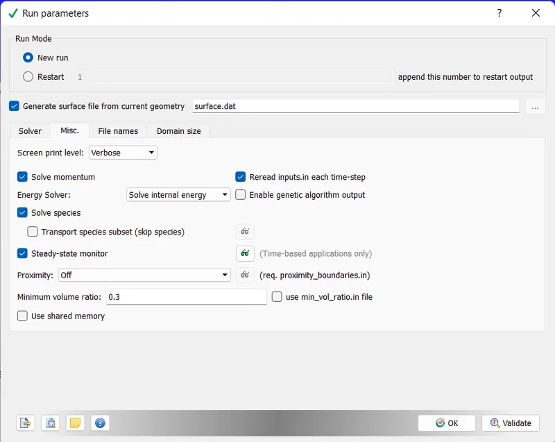
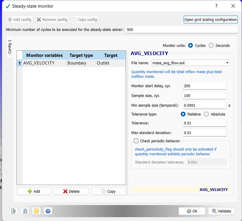
Steady State Monitor, Solve Momentum and Solve Internal Energy , Solve Species option is Enabled.

As it is Steady State we choose for cycles instead of Seconds.Avg.Velocity is choosen as Monitor variable. In converge we have an option to run the simulation for these many number of cycles definitely eventhough the simulation might have reached out convergence limit. This helps us in monitoring furthermore.

The "Monitor Start delay" option allows us to specify the number of cycles after which the monitoring of a variable should begin. This feature is useful for optimizing both space and computational resources on the system, as it enables us to delay the recording of the variable until a certain number of cycles have passed, rather than monitoring it continuously from the beginning of the simulation.

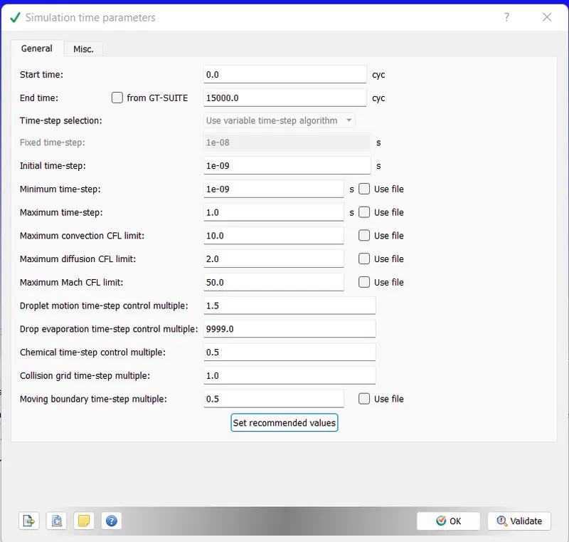
Simulation Parameters has been given here as Start Time=0 Cycles and End Time=15000Cycles with Initial time-step and Min Time-step as 1e-9. Max Time-step as 1.0 and remaining choosen as default values.

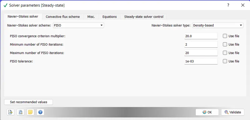
PISO is selected as Navier-Stokes Solver Scheme Algorithm or method, with Density-based Solver type.

4.Boundary Conditions

Boundaries are selecting the faces of Rectangle box. These are represented with Boundary Id's and Name is given for a particular ID.

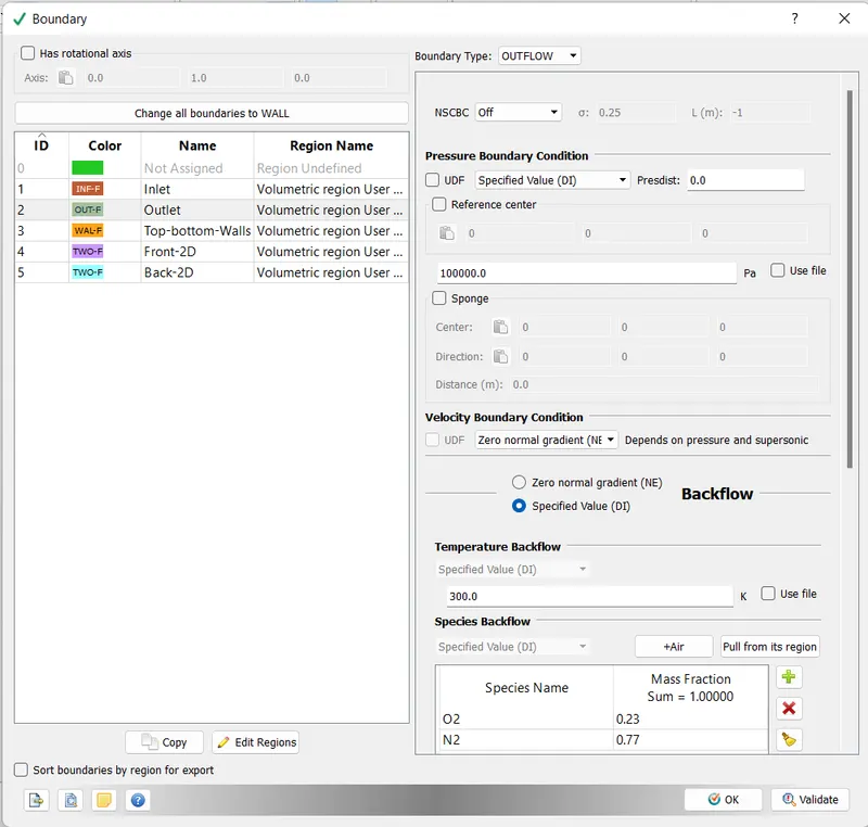
Boundary Id 1 is assigned as Inlet. As flow takes place in X-direction from X=0(Channel Dimension).

Pressure is given as 100001Pascal. And Pressure here is considered as Total Pressure.

And Velocity condition is Normal Neumann.

Species Boundary Condition is given as AIR Assuming only two elements (Components of Premixed Gas-Air). Their Mass Fraction of O2 and N2 are choosen as defaults.

The Normal Neumann boundary condition, also known as the homogeneous Neumann condition, is a type of boundary condition where the derivative of the solution with respect to the outward normal direction is set to zero on the boundary. In the context of fluid mechanics, this condition corresponds to specifying that there is no flow across the boundary.

Therefore, if you have a PDE that describes the behavior of a fluid or a gas, and you specify that the velocity condition is Normal Neumann, it means that you are setting the derivative of the velocity with respect to the outward normal direction to zero on the boundary of the domain. This condition is often used for problems where the flow is confined within a domain and does not cross the boundary.

Pressure Boundary Condition
Specified Value (DI): Dirichlet. Enter a constant value for the static or total (check Total Pressure) pressure at the boundary (Pa) or check Use file to configure a profile.
Zero normal gradient (NE): Neumann. To run the simulation without pressure transfer between the boundary and the fluid, select Zero normal gradient (NE).

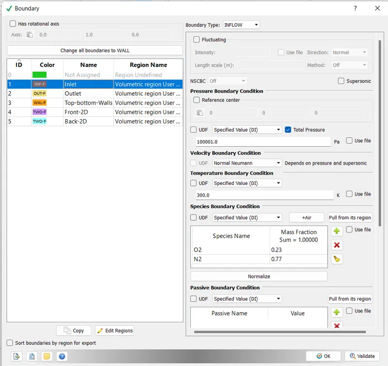
Boundary Id 2 is choosen as outlet and assigned to the region named as Volumetric region user Defined. Pressure is 1Bar and velocity boundary condition is given as Zero Normal Gradient. If there is BackFlow Specified Value(DI) is given with Air as Backflow species material.

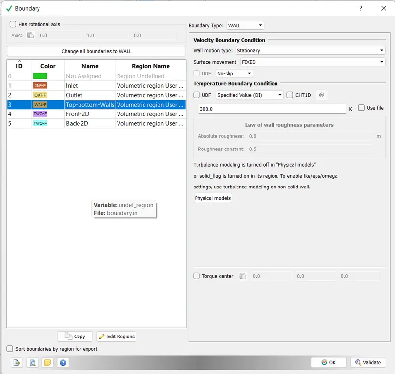
Top & bottom Walls has been choosen as Wall and given Condition of Stationary Wall and FIXED movement with No-Slip Condition is selected Value(DI).

Front and Back Walls are choosen as choosen as 2-D. I assumed that simulation observation is done in 2Dplane that is sufficient. We can match the results of that 2D sliced parts into 3D results which can reduce Computing time.

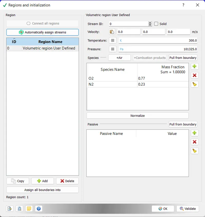
5.Initial Conditions and Events

Here fluid region is selected to perform the required action and to assign that particular region for the flow. And named it as Volumetric region User Defined.

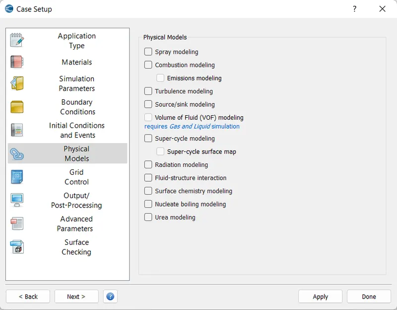
6.Physical Models: No model is choosen in this case.

7.Grid Control- Mesh generation

There is no adaptive mesh refinement is in this case. only Base grid is choosen as default.

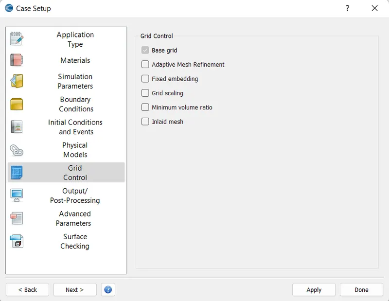
Base grid size is taken as given. Simulation is made for three cases.

• dx = 2e-4m, dy = 2e-4m, dz = 2e-4m
• dx = 1.5e-4m, dy = 1.5e-4m, dz = 1.5e-4m
• dx = 1.0e-4m, dy = 1.0e-4m, dz = 1.0e-4m

8.Output/Post Processing

Post Variable Selection :

From this we can choose type of on which we are looking upon by doing this simulation. Here I selected Pressure, Density , Temperature, Velocity. If there is Turbulence modelling we can choose variables from Turbulance tab.

Output Files:

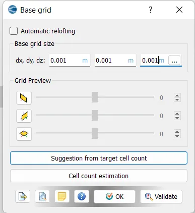
When writing details of the results into a file we can choose how to store that data. There is no need of storing tha data for each and every cycle of solving the simulation. We can given a command after completing how many cycles of simulation the results must be stored. Here I choose for total 15000 cycles of simulation , write a record for every 100 cycles. So that we get almost 150 data files(If simulation reaches convergence limit it may take down for less files). From this we can obtain a clear picture of the flow simulation.

Time Interval for writing Restarting Output file is also choosen as same as Time Interval for 3D output data file.

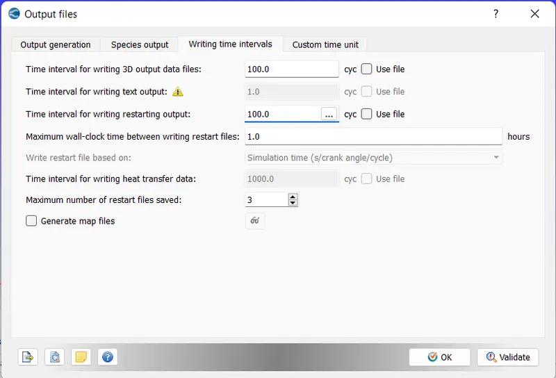
All the above files are exported as Input files into a seperate folder.

To communicate with the CONVERGE solver, we can use a Linux-based command prompt terminal such as CYGWIN. The solver requires input files to be stored in a separate folder, which contain the necessary setup information for the case. Using CYGWIN and the Message Passing Interface (MPI), we can run the case in the CONVERGE solver and store the resulting data in output files (log files), which are saved in the same folder as the input files.

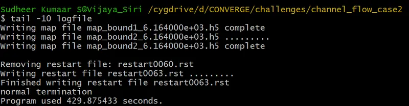
Ran simulation for three cases using the above method and solver timings are mentioned below.

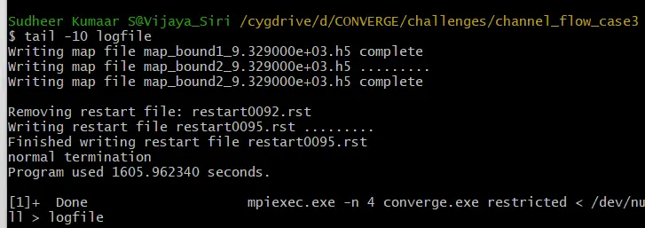
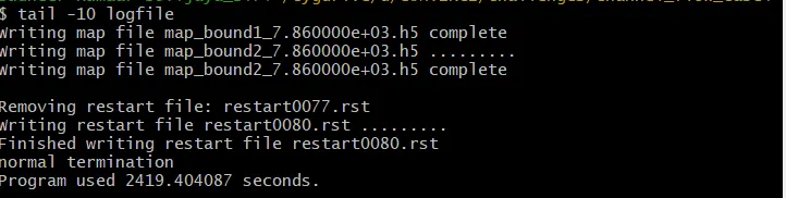
Mesh Element Size (in meters)	Time taken to Solve (in seconds)	Cell Count
2e-4	429.87	25000
1.5e-4	1605.96	45420
1.0e-4	2419.404	100000

The generated output files are converted into Paraveiw readable file format which PARAVIEW VTK In-Line Binary Format. And are stored in the same folder of format ".vtm" group file in output folder.

By using Paraview above cases are analysed for flow contours and plots.

VELOCITY PLOT:

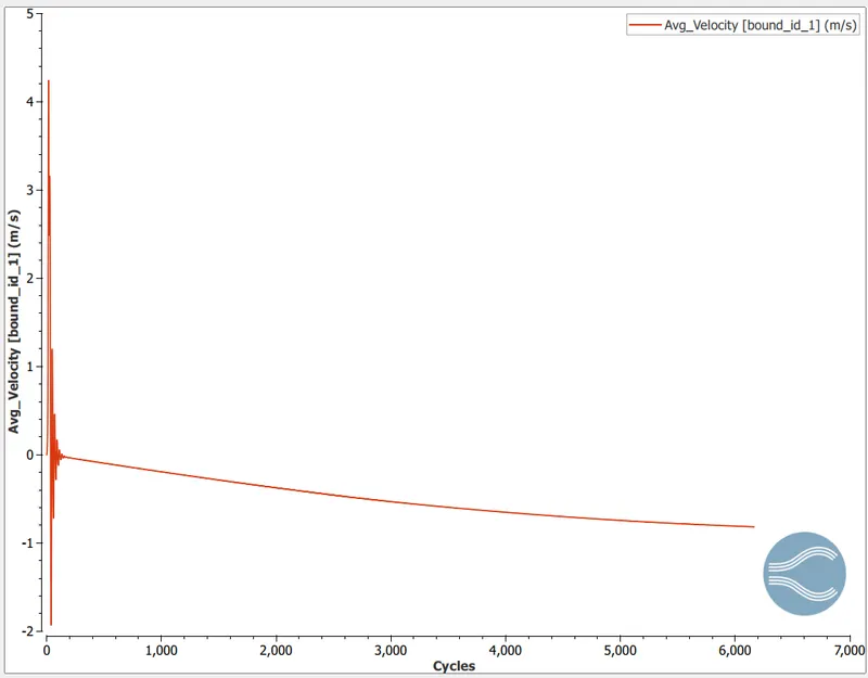
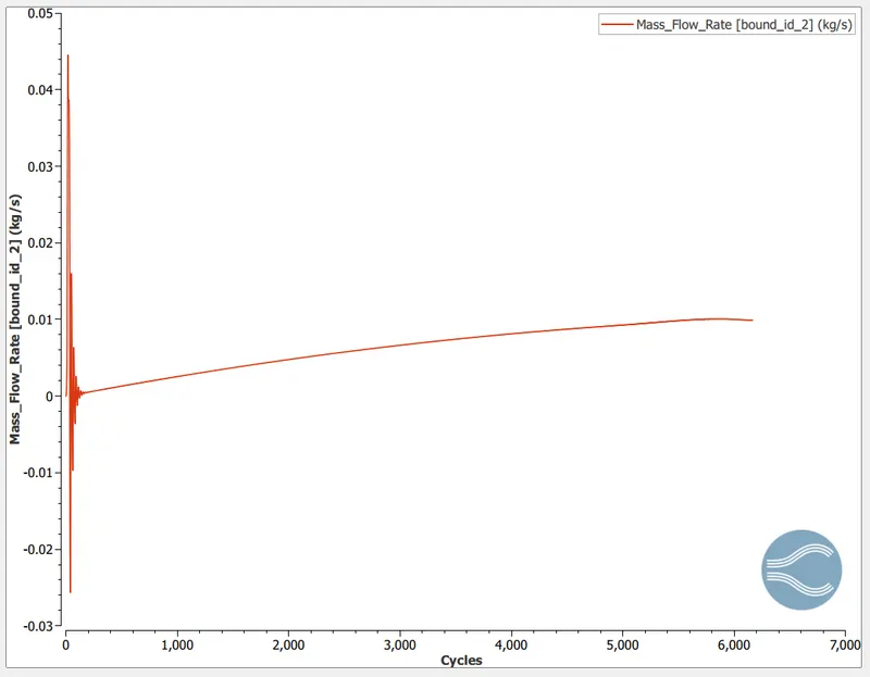
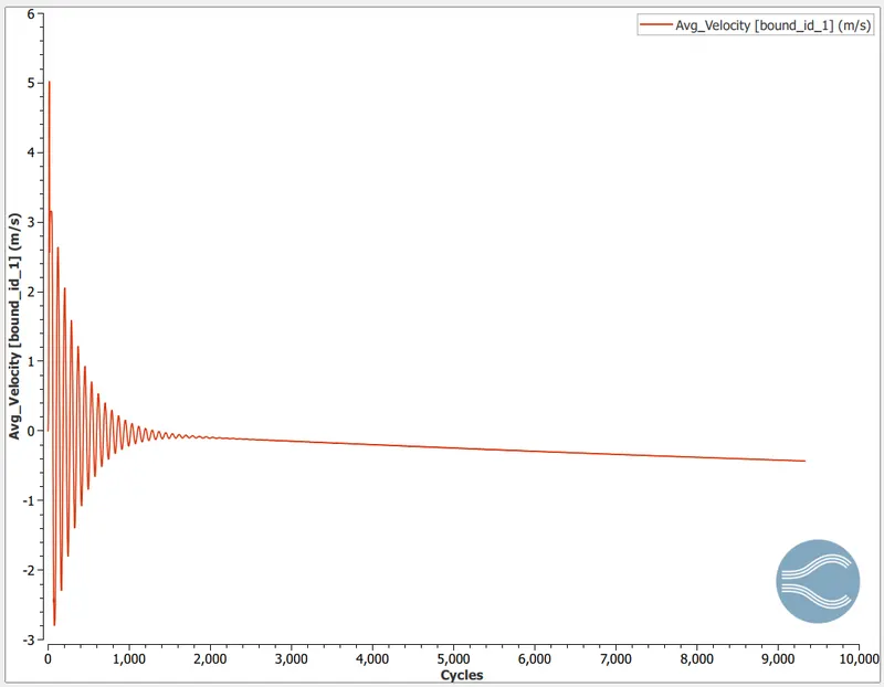
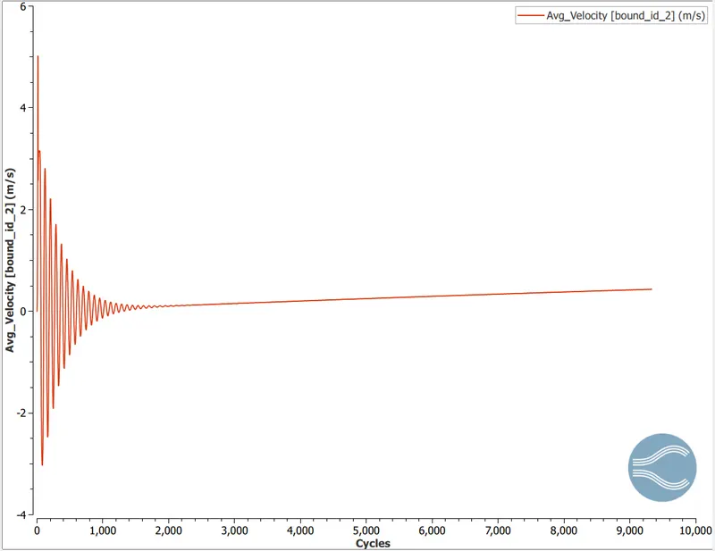
Below were the plots for Inlet and Outlet velocities represented side by side.

For Element size of 2e-4m,

Element size 1.5e-4m

Element Size 1e-4m

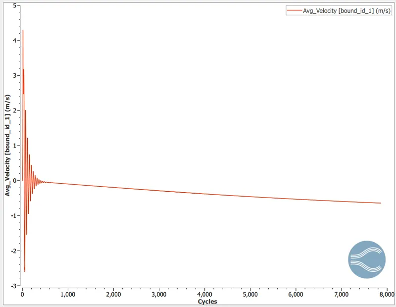
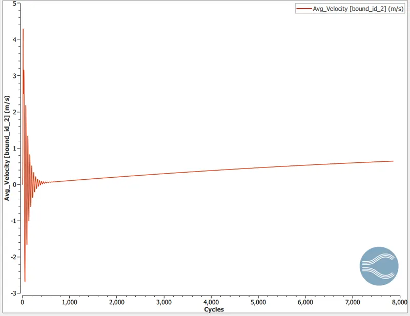
• From velocity plot we can see that for element size 1.5e-4m gave the smooth curve.
• It means that flow is captured properly in that element size.
• Stability in the flow is reached roughly after ~2000cycles.
• Convergence limit has reached at after 6500Cycles in case 1 and ~9500Cycles in case 2 and ~8000cycles in case 3.

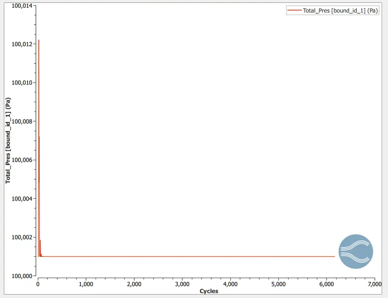
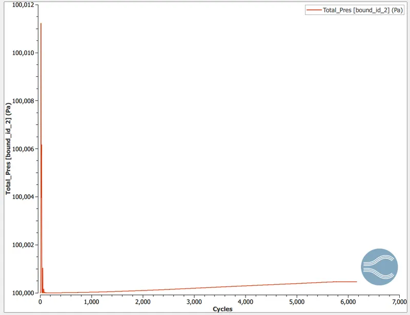
PRESSURE CONTOUR:

For Element size of 2e-4m,

Element size 1.5e-4m

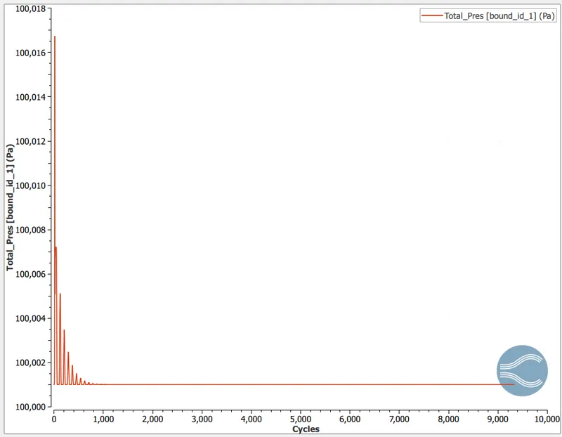
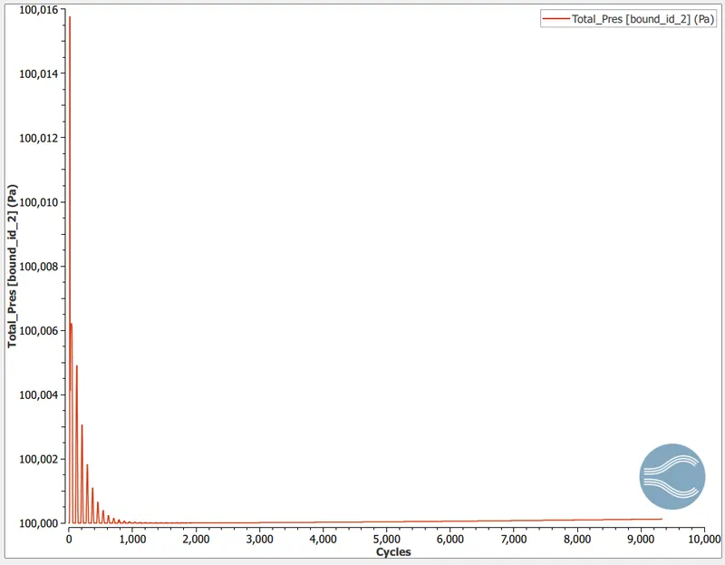
Element Size 1e-4m

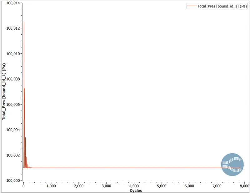
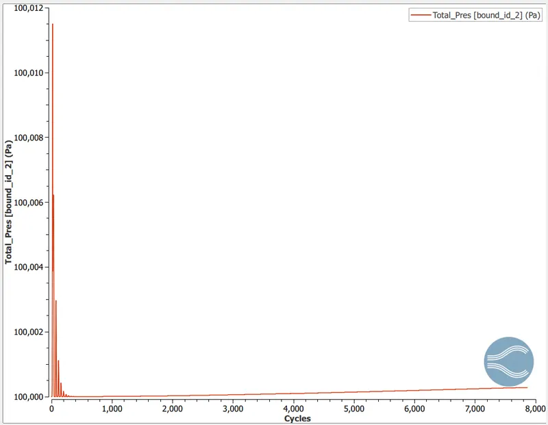
• From Pressure plot we can see that flow happened from high pressure side to low pressure side also for element size 1.5e-4m gave the smooth curve.
• It means that flow is captured properly in that element size.
• Stability in the flow is reached roughly after ~1000cycles.

CONTOURS:

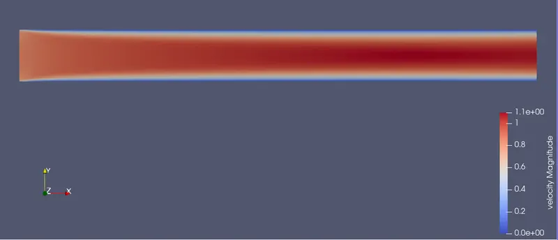
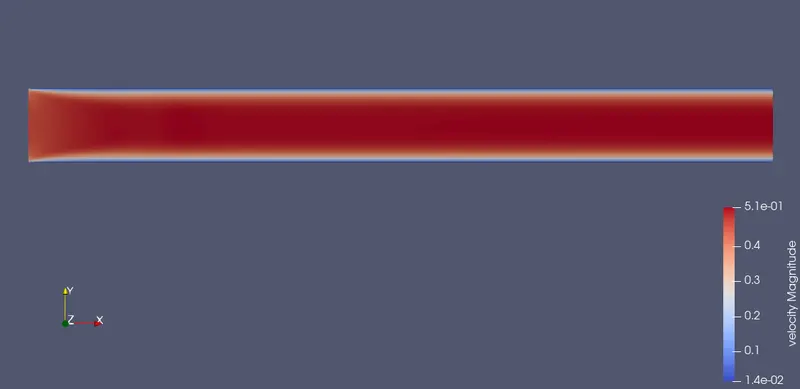
These contours are observed from PARAVIEW used for post-processing stage of CFD. Below are the plots for different elements size.

For Element size of 2e-4m,

Element size 1.5e-4m

Element Size 1e-4m

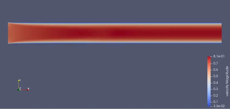
If we observe the plot of second case with Element Size 1.5e-4m is giving us more clear form of flow. Also we can observe that at inlet side flow is uniform and as it is a 2D form of plot at boundary walls of top and bottom walls due to no slip condition we can see the Boundary layer theory in visual. In case 2 it seen more properly.

ANIMATION LINKS:

Element Size 2e-4m

Flow is happened at first based on the Initial conditions which are given in case setup. Later by adopting to the grid parameters and boundary conditions flow is developed and reached convergence..

Element Size 1.5e-4m

Element Size 1e-4m

CONCLUSION:

• From the above simulation we can observe that for Element Size 1.5e-4m we got the flow visualization and observation of flow behaviour of the fluid properly.
• Also, CONVERGE gave us more flexible kind of approach in solving CFD simulation in the form of Setting up the case and Solving and also in Post-Converting the simulation.