1. Plot a function y(x) = (x-1) * (x-3)^2 * (x-9)^2 using basic Simulink blocks.

2. Run Simulink example “Suspension System Comparison” and answer the following:

1. 1. What is the objective of the simulation? What are the similarities and differences between the three systems understudy?
   2. What are your observations from the results?
   3. How the oscillating velocity source is created?

Grading Policy :

1. Upload the supporting results as images or by any other means

2. Write a detailed report

3. Report attached as an image will lead to zero marks

4. plagiarism is not tolerated

5. upload Simulink files if needed through the google drive, any external links will not be accepted

Objective : To plot a function y(x)=(x-1)*(x-3)^2*(x-9)^2 using basic Simulink blocks.

Matlab Simulink Description:

Simulink is a block diagram environment for multidomain simulation and Model-Based Design. It supports system-level design, simulation, automatic code generation, and continuous test and verification of embedded systems. Simulink provides a graphical editor, customizable block libraries, and solvers for modeling and simulating dynamic systems.

Model-Based Design with Matlab:

Modeling is a way to create a virtual representation of a real-world system. You can simulate this virtual representation under a wide range of conditions to see how it behaves.

Modeling and simulation are valuable for testing conditions that are difficult to reproduce with hardware prototypes alone. This is especially true in the early phase of the design process when the hardware is not yet available. Iterating between modeling and simulation can improve the quality of the system design early, by reducing the number of errors found later in the design process.

We can automatically generate code from a model and, when software and hardware implementation requirements are included, create test benches for system verification. Code generation saves time and prevents the introduction of manually coded errors.

In Model-Based Design, a system model is at the center of the workflow. Model-Based Design enables fast and cost-effective development of dynamic systems, including control systems, signal processing systems, and communications systems.

Model-Based Design allows us to:

• Use a common design environment across project teams

• Link designs directly to requirements

• Identify and correct errors continuously by integrating testing with design

• Refine algorithms through multidomain simulation

• Automatically generate embedded software code and documentation

• Develop and reuse test suites

Simulink Block Diagram:

Simulink is a graphical modeling and simulation environment for dynamic systems. You can create block diagrams, where blocks represent parts of a system. A block can represent a physical component, a small system, or a function. An input/output relationship fully characterizes a block.

The definition of a block is only complete with its inputs and outputs defined; this task relates to the goal of the model. Simulink provides block libraries that are collections of blocks grouped by functionality. We can connect blocks to other blocks to form systems and represent more complex functionality.

The primary function of Simulink is to simulate the behavior of system components over time. In its simplest form, this task involves keeping a clock, determining the order in which the blocks are to be simulated and propagating the outputs computed in the block diagram to the next block.

Simulink handles data in three categories:

• Signals — Block inputs and outputs, computed during the simulation

• States — Internal values, representing the dynamics of the block, computed during the simulation

• Parameters — Values that affect the behavior of a block, controlled by the user

Introduction to Open New Model in Simulink

Use of the Simulink Editor to build our models.

1. Start From the MATLAB toolstrip, click the Simulink button

1. 

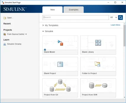
Fig - Simulink Start Page

2. Click the Blank Model template. The Simulink Editor will get open.

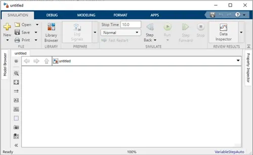
Fig - Blank Model Template

3. From the Simulation tab, select Save > Save as. In the File name text box, enter a name for your model. For example, Click Save. The model is saved with the file extension “.slx.”

Open Simulink Library Browser

Simulink provides a set of block libraries, organized by functionality in the Library Browser. The following libraries are common to most workflows:

• Continuous — Blocks for systems with continuous states

• Discrete — Blocks for systems with discrete states

• Math Operations — Blocks that implement algebraic and logical equations

• Sinks — Blocks that store and show the signals that connect to them

• Sources — Blocks that generate the signal values that drive the model

1. From the Simulation tab, click the Library Browser button
2. To browse through the block libraries, select a category and then a functional area in the left pane. To search all of the available block libraries, enter a search term.

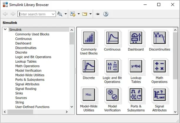
Fig - Simulink Library Browser

Input:

Here we have to plot the function as given below using basic MATLAB Simulink block

`y(x) = (x - 1) × 〖(x - 3) 〗^2× 〖(x - 9)〗`

To make this we have to use various block which is already inbuilt in MATLAB Simulink. Various blocks which have been used as input are mentioned below as -

1) Ramp

2) Constant

3) Sum

4) Square

5) Product

6) Display

7) Scope

Description of block :

Ramp - The Ramp block generates a signal that starts at a specified time and value and changes by a specified rate. The block's Slope, Start time and Initial output parameters determine the characteristics of the output signal.

Constant - The Constant block generates a real or complex constant value signal.

Sum - Actually this is the block for addition & subtraction of element but in our case, we used it for subtraction purpose.

Square - The square block will square the input element.

Product - This block takes the input element and performs the multiplication of the input provided to it.

Display - It displays the final result of the model for which the model is been prepared.

Scope - This block is used to see the result of the model in terms of graph or plot.

With the help of all the above-mentioned blocks, the function is represented in the image below using Matlab Simulink.

Representation :

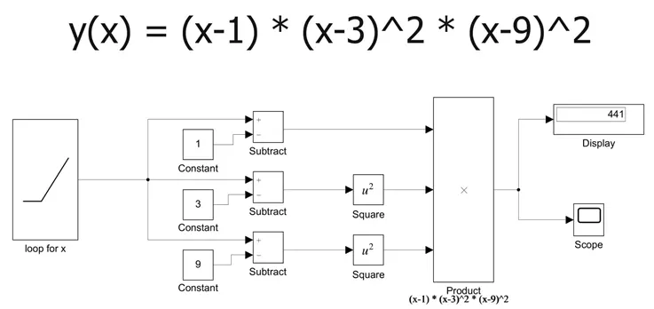
Fig - Simulink Model of Mathematical Model

Output result using the scope :

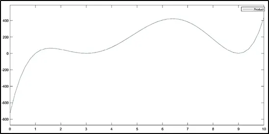
Fig - Output nature of a given mathematical model

Here we can see from the graph that as the value of 'x' changes for the time the value of product changes respectively.

Conclusion - By solving this Simulink model we can say that how Simulink makes it easier to build a mathematical model in its environment.

2.Suspension System Comparison

AIM:

To create a block diagram using Simulink for better comparison and understanding of suspension system using in vehicle

OBJECTIVES OF THE SIMULATION:

This simulation shows a testbed containing three sets of springs and dampers excited by the same oscillating velocity source.

To compare the three plots like (shock absorber,Non linear spring, varaiable spring) and analysis the good suspension system.

SUSPENSION SYSTEM:

Suspension is the system of tires, tire air, springs, shock absorber and linkages that connects a vehicle to its wheels and allows relative motion between the two. Suspension systems must support both road holding/handling and ride quality, which are at odds with each other. The tuning of suspensions involves finding the right compromise. It is important for the suspension to keep the road wheel in contact with the road surface as much as possible, because all the road or ground forces acting on the vehicle do so through the contact patches of the tires.

Sprung weight transfer:

Sprung weight transfer is the weight transferred by only the weight of the vehicle resting on the springs, not the total vehicle weight. Calculating this requires knowing the vehicle's sprung weight (total weight less the unsprung weight), the front and rear roll center heights and the sprung center of gravity height (used to calculate the roll moment arm length). Calculating the front and rear sprung weight transfer will also require knowing the roll couple percentage.

Unsprung weight transfer:

Unsprung weight transfer is calculated based on the weight of the vehicle's components that are not supported by the springs. This includes tires, wheels, brakes, spindles, half the control arm's weight and other components. These components are then (for calculation purposes) assumed to be connected to a vehicle with zero sprung weight. They are then put through the same dynamic loads. The weight transfer for cornering in the front would be equal to the total unsprung front weight times the G-Force times the front unsprung center of gravity height divided by the front track width. The same is true for the rear.

OSCILLATING VELOCITY SOURCE:

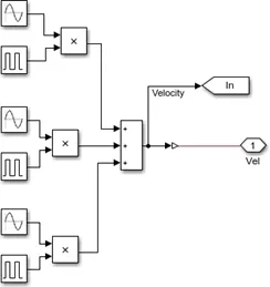
Oscillating velocity source is created by the flow chart that are given above. An sine wave and pulse generator are produced an new velocity of x . Same process are acted in another two blocks and the three blocks are calculated in sum block.

Final output values are assigned as input values for velocity that will passed in three systems.

INPUT:

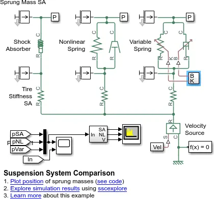
Similarities and differences between the three systems understudy

An velocity source appiled here is considered as input of all three systems. Tire stiffness, sprung mass and unsprung mass are also similar for all three systems.

Sprung mass is total mass that depends upon the spring and Unsprung mass is a mass that doesn't depends upon the spring.

The difference between the three systems are explained below,

The first uses the Shock Absorber block and includes linear stiffness and damping. Optional friction and hard stops are not used.

The second shock absorber uses a Nonlinear Translational Spring and a Nonlinear Translational Damper specified by symmetric polynomials.

The third uses a Variable Translational Spring and Variable Translational Damper.

B . Observations from the results:

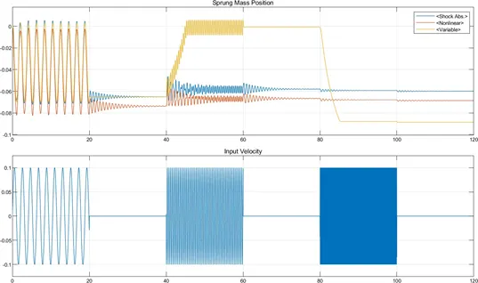
The three different sysytems are perform to find better suspension system or to compare different system output performance.

Inputs are equally distributed for each systems by velocity source. spring and tire stiffness transmit the energy source to different sytems.

In shock absorber the damping is done that reduces the vibration during the oscillation of the velocity. Optional friction and hard stops are not used.

The Nonlinear Translational Spring consists of unequal spring due to this there will be less displacement is acted.

Varaiable spring the damping absorbtion is low due to variation in coil pitch. And duration of stiffness are taking long time this causes variation in displacement to lower level to higher level.

COMPARISON OF THREE SYSTEM:

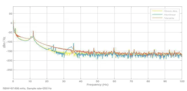
These graphs shows the input velocity and variation in the sprung mass positions of three systems,

The shock absorber act as the linear displacement by the duration of time. shock absorber reduces the vibration from the actual input velocity. That shows reduction of oscillation. Data of output are colllected in pSA to plot the graph and

compare with the other system.

Nonlinear Translational Spring act as less dispacement due to the unequal coil the velocity of input are not acted completely. Data of output are colllected in pNL to plot the graph and compare with the other system.

Varaiable spring are conical spring that varies with the coil pitch due to this suspension process takes more duration of time and stiffness also not stable it may changes from low to high displacement. Data of output are colllected in pVar to plot the graph and compare with the other system.

CONCLUSION:

Thus comparing with all three suspension system shock absorber system seems good stiffness and displacement are present, vibration is also low in this system. The nonlinear spring are similar to the shock absorber but the stiffness is low. And the variable spring seems a bad performance due to duration of stiffness time. The vibrations are varies in each time .Sudden

raises and lowerd are also occur so it is considered as poor system.

Therefore performance of shock absorber is high than the other two suspension system.