vehicle dynamics week 5
1-combined slip:
Matlab code:
clear all
close all
clc
fz = 4000;
mu = 0.85;
lt = 0.2;
kt = 3500000;
ky = 2500000
cs=0.5*kt*(lt)^2
ca=0.5*ky*(lt)^2
alpha=linspace(2,10,5)
sr=linspace(0,1,100)
for j=1:length(alpha)
alpha_rad=alpha(j)*(pi/180)
for i=1:length(sr)
lc =((mu*fz)*(1-sr(i))*lt)/((2*sqrt(((cs*sr(i))^2)+(ca*tan(alpha_rad))^2)))
if lt<lc
fx(i,j)=(cs*sr(i))/(1-sr(i))
fy(i,j)=(ca*tan(alpha_rad))/(1-sr(i))
else
fx(i,j)=((mu*fz*cs*sr(i))/(((cs*sr(i))^2+(ca*tan(alpha_rad))^2)^0.5))*(1-((mu*fz*(1-sr(i))/(4*((((cs*sr(i))^2)+((ca*tan(alpha_rad))^2))^0.5)))))
fy(i,j)=((mu*fz*ca*tan(alpha_rad))/(((cs*sr(i))^2+(ca*tan(alpha_rad))^2)^0.5))*(1-((mu*fz*(1-sr(i)))/(4*((((cs*sr(i))^2)+((ca*tan(alpha_rad))^2))^0.5))))
end
i=i+1
end
j=j+1
end
plot(fx,fy,'linewidth',2)
grid on
steps:
-inputs are declared
-cs calculated using 0.5*kt*lt^2
-Ca calculated using 0.5*ky*lt^2
-then alpha is declared from 2 to 10 with 5 steps in between
-then slip ratio is declared from 0 to 1 with 100 steps in between
-then for loop is started with counter “j” which has same length as alpha array
-then alpha radian is defined
-then another loop is started with counter I which has same length as slip ratio
-Then critical length is defined which is equal (mu*fz*(1-slip ratio)*lt)/2sqrt((cs*slipratio)^2+ca*tan(alpha)^2)
-then if condition is established ,if lt is smaller than the critical length then :
Fx=slipratio*cs/1-slip ratio
Fy=ca*tan(alpha)/1-slipratio
-if lt is greater than the critical length then:
Fx=(mu*fz*cs*slip ratio)/((cs*slip ratio)^2+ca*tan(alpha)^2)^0.5*[1-mu*fz*(1-slipratio)/4*((cs*is)^2+(ca*tan(alpha))^2)^0.5
Fy=(mu*fz*csa*tan(alpha))/((cs*slip ratio)^2+ca*tan(alpha)^2)^0.5*[1-mu*fz*(1-slipratio)/4*((cs*is)^2+(ca*tan(alpha))^2)^0.5
-then fx and fy is plotted
Combined slip theory:
the tyre can only generate certain forces in the longitudinal or lateral direction and any combination between the two will result in resultant force with lower value in each direction
plot:
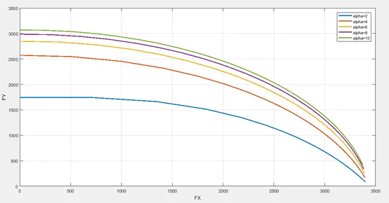
The plot clearly shows the effect of combined slip, as it shows that as the longitudinal force is increased, the lateral force is reduced, and vice versa, it also shows that higher slip angles results in higher lateral loads which is logical.
2-Effective cornering stiffness:
Matlab code:
clear all
close all
clc
fz = 3000;
mu = 0.8;
lt = 0.2;
kt = 4e6;
ky = 2.275e6
cs=0.5*kt*(lt)^2
ca=0.5*ky*(lt)^2
alpha=3
alpha_rad=alpha*(pi/180)
sr=[0:0.005:1]
for i=1:length(sr)
lc =((mu*fz)*(1-sr(i))*lt)/((2*sqrt(((cs*sr(i))^2)+(ca*tan(alpha_rad))^2)))
if lt<lc
fx(i)=(cs*sr(i))/(1-sr(i))
fy(i)=(ca*tan(alpha_rad))/(1-sr(i))
c_eff(i)=fy(i)/alpha_rad
else
fx(i)=((mu*fz*cs*sr(i))/(((cs*sr(i))^2+(ca*tan(alpha_rad))^2)^0.5))*(1-((mu*fz*(1-sr(i))/(4*((((cs*sr(i))^2)+((ca*tan(alpha_rad))^2))^0.5)))))
fy(i)=((mu*fz*ca*tan(alpha_rad))/(((cs*sr(i))^2+(ca*tan(alpha_rad))^2)^0.5))*(1-((mu*fz*(1-sr(i)))/(4*((((cs*sr(i))^2)+((ca*tan(alpha_rad))^2))^0.5))))
c_eff(i)=fy(i)/alpha_rad
end
i=i+1
end
c_report=[c_eff(find(sr==0)),c_eff(find(sr==0.15)),c_eff(find(sr==1))]
figure(1)
plot(sr,fy,'linewidth',2)
grid on
figure(2)
plot(fx,fy,'linewidth',2)
grid on
figure(3)
plot(sr,fx,'linewidth',2)
grid on
steps
inputs are declared
-cs calculated using 0.5*kt*lt^2
-Ca calculated using 0.5*ky*lt^2
-then alpha is inputted
-then alpha radian is defined
-then slip ratio is declared from 0 to 1 with 0.005 steps in between
-then alpha radian is defined
-then loop is started with counter I which has same length as slip ratio
-Then critical length is defined which is equal (mu*fz*(1-slip ratio)*lt)/2sqrt((cs*slipratio)^2+ca*tan(alpha)^2)
-then if condition is established ,if lt is smaller than the critical length then :
Fx=slipratio*cs/1-slip ratio
Fy=ca*tan(alpha)/1-slipratio
-Then cornering stiffness is defines as fy/alpha
-if lt is greater than the critical length then:
Fx=(mu*fz*cs*slip ratio)/((cs*slip ratio)^2+ca*tan(alpha)^2)^0.5*[1-mu*fz*(1-slipratio)/4*((cs*is)^2+(ca*tan(alpha))^2)^0.5
Fy=(mu*fz*csa*tan(alpha))/((cs*slip ratio)^2+ca*tan(alpha)^2)^0.5*[1-mu*fz*(1-slipratio)/4*((cs*is)^2+(ca*tan(alpha))^2)^0.5
- Then cornering stiffness is defines as fy/alpha
-then c_report array is made by making matlab identify the cornering number of element which has slip ratio =0,0.15,1 using “find” command ,then filing the array with cornering stiffness value from the cornering stiffness array which has the same number
-then figure 1 is plotted which has slip ratio and fy
-then figure 2 is plotted which has fx and fy
-then figure 3 is plotted which has slip ratio and fx
cornering stiffness values:
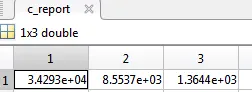
Effecting cornering stiffness at 0 slip ratio=3.420*10^4 N/rad
Effective cornering stiffness at 0.15 slip ratio =8.5537*10^3 N/rad
Effective cornering stiffness at 1 slip ratio=1.3644*10^3 N/rad
plots:
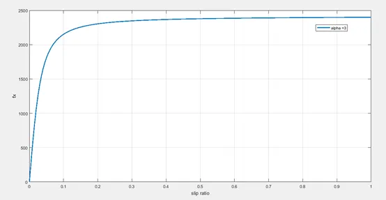 slip ratio-fx curve
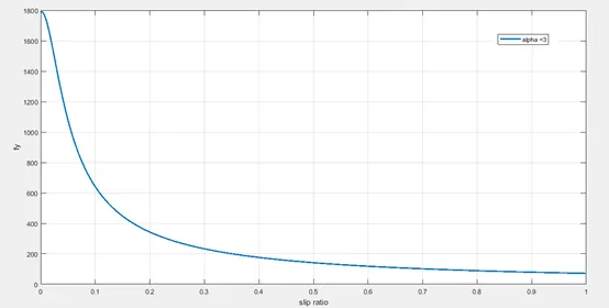 slip-ratio FY curve
Th plot shows that the optimal region for best longitudnal force and good lateral force occurs at slip ratio os 0.15 that's why it is used with abs as it provides very high sopping force while at the same time, provides a good lateral force for steerability during braking.
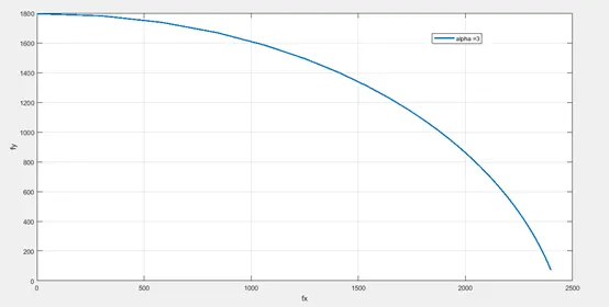 combined slip curve at 3 angle
this plot shows the same phenomena discussed in the previous task
3-pacjecka tyre formula:
Matlab code:
clear all
close all
clc
d_int=58
xm_int=3.36
c_int=2.18
slope_int=27
shz_int=0
svz_int=0
b_int=slope_int/(c_int*d_int)
e_int=((b_int*xm_int)-tan(pi/(2*c_int)))/((b_int*xm_int)-atan(b_int*xm_int))
load tire_test_data
alpha=tire_test_data(:,1)
mz=tire_test_data(:,2)
plot(alpha,mz,'o')
hold on
b = 0.2;
c= 2.18;
d= 59;
e= -2.5;
shz= 0;
svz= 0;
for i=1:length(alpha)
ALPHA(i)=(alpha(i))+shz
Mz(i)=d*sin(c*atan((b*ALPHA(i)-e*(b*ALPHA(i)-atan(b*ALPHA(i))))))
MZ(i)=Mz(i)+svz
diff(i)=(MZ(i)-mz(i))^2
i=i+1
end
RMSE = sqrt(mean(diff))
plot(ALPHA,MZ,'linewidth',3)
grid on
steps:
Input parameters:
b = 0.2;
c= 2.18;
d= 59;
e= -2.5;
shz= 0;
svz= 0;
steps:
-Initial parameters are inputted, these parameters are known from iterations and through equations like B=slop/D and E=(B*Xm-tan(pi/2*c))/(B*Xm-arctan(B*Xm)
-then tyre test data is loaded
-then all the elements in the first column is inputted in array called alpha
-then all the elements in the second column is inputted in an array called mz
-then the test data is plotted and hold on command is used to plot in the next steps the computed data on the same plot
-then for loop is started which have the same length as the alpha from test data
-then the shz is added to alpha
-then moment is calculated using d*sin(c*atan(b*alpha-e*(b*alpha-atan(b*alpha)))
-then moment is added to svz
-then in order to establish the root mean square error first the square error part is computed by subtracting the computed moment form test moment and squaring it and storing it in diff array
-then mean part is computed using the ‘mean function’ which adds all the squared error in the diff array and divides it by the number of elements, then the last step it is squares in order to get root mean square error
-Then the computed moment is plotted with alpha
Magic formula theory:
magic formula is an empirical tyre model which has no physical basics and it is averaged from experiments and it fit a wide variety of tire constructions and operating conditions. Each tire is characterized by 10–20 coefficients for each important force that it can produce at the contact patch, typically lateral and longitudinal force, and self-aligning torque, as a best fit between experimental data and the model.
plot:
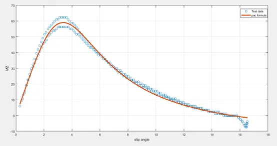
the curve fits the experimental data which is taken in two directions
RMSE:
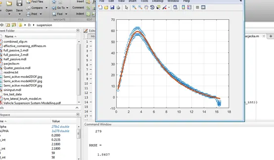
RMSE=1.8607
Files:
combined slip:
https://drive.google.com/file/d/1CjN2a0IEQYiFR-BYShKImxDzm0hUvjAW/view?usp=sharing
Effective cornering stiffness:
https://drive.google.com/file/d/15KGOpPPk3MC185hx5GdSRk1k4JIDTrV3/view?usp=sharing
Pacjecka:
https://drive.google.com/file/d/1ZQgMQ7qlB7mvx4tI5NS6HW8-fCtC9i49/view?usp=sharing