vehicle dynamics week 4

Questions:

1a, These questions test conceptual knowledge. Answer in a sentence or two in your own words. A textbook definition is not necessary
(2 points each for a total of 10 points)

• Calculate the tire stiffness. Tire size – 275/40R18, Free radius is 13.33 inches and loaded radius is 12.36 inches
• Explain in your own words what slip ratio and slip angle are (explain, don’t give the formula)
• What is the risk of having too much mechanical trail? (think in terms of driving at the limit)
• You know lateral force is proportional to slip angle. Can a tire produce lateral force at zero slip angle?
• In your own words, explain tire load sensitivity and how increasing the rear roll bar size can induce oversteer (again, use your own words)

Answers:

-Tyre stiffness can’t be calculated because the load on the tyre is unknown, if it is known: ktyre=fz (load)/(free radius-loaded radius)

-rubber provides forces by stretching and sliding,The difference between the distance the wheel should have covered if the rubber at the contact patch wasn't 'stretching and sliding' and the actual distance that the car has covered (with all this sliding) dividing it by time to get the velocity and then expressing it as a percentage, is the 'slip ratio'.,

Slip angle:tyre can offer resistance to lateral force by stretching and slipping,so this results difference between the actual direction of travel and the direction which the tyre is pointing (which the tyre should follow if there is no deformation in the rubber) ,this difference is called the slip angle.

-it can dilute the pneumatic trail which is an indicator of the grip available at the tyre contact patch which gives the driver early warning of any loss of grip occurring at the contact patch through reduction of steering resistive torque which is felt by the driver, so ahigh mechanical trail can dilute this feedback which can result in a driver losing control of the vehicle due to insufficient early warning.

-yes, tyre can produce lateral force at zero slip angle when it is cambered which is called camber thrust and it is used mainly by motorbikes to generate cornering forces

-tyre load sensitivity describes the tyre behavior under vertical load, Coulomb friction theory says that the maximum horizontal force developed should be proportional to the vertical load on the tire. In practice, the maximum horizontal force Fy that can be generated by a tyre is proportional, roughly, to the vertical load Fz raised to the power of somewhere between 0.7 and 0.9.so the lateral force generated by the tyre is increased with vertical load but at diminishing rate and it has a limit,increasing anti roll bar stiffness in the rear will increase the load transfer portion to the rear which will results that this axle will be losing more grip on the unloaded tyre(in linear region) than it is gaining on the loaded tyre (more in plateau region) which will result in the rear axle losing grip before the front axle resulting in oversteer on the other hand,the front axle will have lower load transfer to deal with ,so it will be have more grip regained on the loaded tyre compared (more in linear region) to the rear axle so it can more effectively counter the loss of grip of the unloaded tyre (in linear region).

part 2: Matlab code:

clear all

close all

clc

mu=0.9

fz=5000

lt=0.2

ca=50000

ky=(2*ca)/(lt)^2

alpha_c=(mu*fz)/(2*ca*(pi/180))

alpha=linspace(0,15,150)

for i=1:length(alpha)

alpha_rad(i)=alpha(i)*(pi/180)

if alpha(i)<alpha_c

fadh(i)=ca*alpha_rad(i)

mzadh(i)=(ca*lt*alpha_rad(i))/6

else

fadh(i)=(mu*fz)-((mu*fz)^2/(4*ca*tan(alpha_rad(i))))

mzadh(i)=(((mu*fz)^2)/(12*lt*ky*tan(alpha_rad(i))))*(3-((2*mu*fz)/((lt^2)*ky*tan(alpha_rad(i)))))

end

i=i+1

end

subplot (1,2,1)

plot(alpha,fadh)

grid on

hold on

subplot(1,2,2)

plot(alpha,mzadh)

grid on

steps:

-inputs are declared

-Ky is calculated using ky=2*ca/(lt)^2

-then critical angle is calculated using (mu*fz/(2*ca*(pi/180))

-then alpha is declared from zero to 15 with 150 point in between

-then for loop is set with counter starting from 1 and ending when the alpha array ends (has the same value as number of elements in alpha array)

-then if alpha radian is defined

-then if condition is set which states that if the slip angle is lower than the critical angle,

-Fy=ca*alpha

-Mz=(ca*lt*alpha)/6

-Then if it is higher than the critical angle then:

Fy=mu*fz-((mufz)^2/4*ca*tan (alpha))

Mz=((mu*fz)^2/12*lt*ky*tan(alpha))*[3-2*mu*fz/lt^2*ky*tan(alpha)]

-Then the two plots is drawn in the same figure using the subplot command

plots:

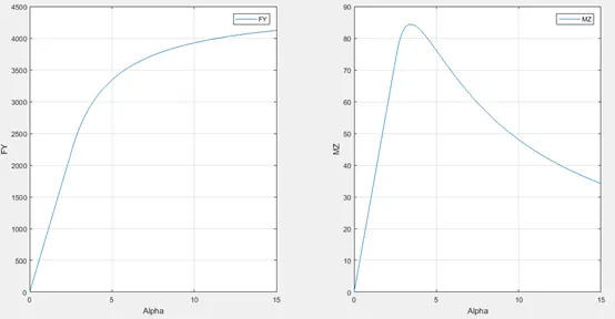
The slip angle shows that cornering force first increases linearly and and then it starts reaching a plateau which will mean that after that the tyre will start sliding and increasing slip angle will not result in any increase in cornering force (it can actually decrease),the moment diagram shows that that it reaches peak nearly at the same point as the end of the linear region of the slip angle curve,this means that at this instant micro sliding starts (non linear region begin) occuring in regions of the contact patch which result in reducing the pneumatic trail which reduces the aligning moment even despite the slight increase in lateral force generated at higher slip angles,this can give the driver critical feedback by reducing the resistive torque in the steering before the vehicle actually loses its grip, so the driver can take action at the right time.

files:

questions:

https://drive.google.com/file/d/1eNH1l5YP_1aqFxpl6EB05CxJ_bEz2emO/view?usp=sharing

matlab file:

https://drive.google.com/file/d/1sBd4m5ms7gT_CYchh_rbmS2Vi3J_ErSc/view?usp=sharing