vehicle dynamics week 11C
Question:
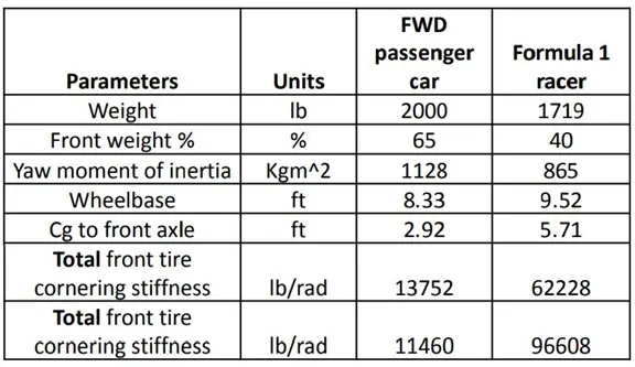
. Calculate the following parameters for both using formulas
- Undamped natural frequency (Hz) (3 points)
- Damping ratio (3 points)
- Damped frequency (Hz) (2 points)
- Rise time(2 points)
- Plot the unit step response of the system for lateral speed, lateral acceleration and yaw rate (5 points)
- Plot the sine response of for lateral speed, lateral acceleration and yaw rate (5 deg, 7hz sine input) (10 points)
- Plot the yaw gain (yaw/steering input) in the frequency domain (5 points)
- Show correlation for the following (in other words, you should get the same answer between two different methods of calculation) (15 points)
- Steady state yaw gain - between the sine response and the frequency response plot
- Yaw gain at 7hz - between the sine reponse and the frequency response plot
- Response time - between the step response plot and your analytical calculations
FWD code:
clear all
close all
clc
l = 2.538984 ; % Wheelbase (m)
a = 0.890016; % cg to front axle (m)
b = l-a; % cg to rear axle (m)
m = 907.18474; % Mass (kg)
jz = 1128 ; % moment of inertia (kg-m^2)
cf = 61171.9437; % front cornering stiffness (N/rad)
cr = 50976.6191; % rear cornering stiffness (N/rad)
u = 100/3.6; % m/s
A=[-(cf+cr)/(m*u),(((b*cr)-(a*cf))/(m*u))-u;((b*cr)-(a*cf))/(jz*u),-((((a^2)*cf)+((b^2)*cr))/(jz*u))]
B=[cf/m;(a*cf)/jz]
c1=[1,0] %lateral speed
d1=0
c2=[0,1] % yaw rate
d2=0
c3=A(1,:)+u*[0,1] %lateral acceleration
d3=B(1)
t=[0:0.01:2]
st=(pi/180)*5*sin(2*pi*7*t)
C=[c1;c2;c3]
D=[d1;d2;d3]
sys=ss(A,B,C,D)
Y=lsim(sys,st,t)
sys.Inputname={'st'}
sys.Outputname={'lateral speed','yaw rate','lateral acceleration'}
[mag1,phase1,omega1] = bode(sys({'yaw rate'},{'st'}))
for i=1:length(mag1)
magnitude1(i)=mag1(1,1,i)
i=i+1
end
figure(1)
loglog(omega1/(2*pi),magnitude1,'linewidth',2)
title('yaw gain frequency response')
grid on
grid on
figure(2)
subplot(2,2,1)
plot(t,st,'linewidth',2)
title('steering')
grid on
subplot(2,2,2)
plot(t,Y(:,1),'linewidth',2)
title('lateral speed')
grid on
subplot(2,2,3)
plot(t,Y(:,2),'linewidth',2)
title('yawrate')
grid on
subplot(2,2,4)
plot(t,Y(:,3),'linewidth',2)
title('lateral accelaration')
grid on
figure(3)
step(sys)
grid on
S=stepinfo(sys)
[wn theta]=damp(sys)
Cf = -61171.9437; % front cornering stiffness (N/rad)
Cr = -50976.6191
YB=Cf+Cr
YR=(a*Cf-b*Cr)/u
YS=-Cf
NB=a*Cf-b*Cr
NR=(((a^2)*Cf)+((b^2)*Cr))/u
NS=-a*Cf
Wn=sqrt(((YB*NR)+(NB*m*u)-(YR*NB))/(m*u*jz))
Theta=abs(-((NR/jz)+(YB/(m*u)))*(1/(2*Wn)))
Wd=Wn*sqrt(1-(Theta)^2)
tr=((m*u*NS)/((YS*NB)-(YB*NS)))
Steps:
-first input is declared
-then A matrix is inputted using A=[-(cf+cr)/(m*u),(((b*cr)-(a*cf))/(m*u))-u;((b*cr)-(a*cf))/(jz*u),-((((a^2)*cf)+((b^2)*cr))/(jz*u))]
-then b matrix is inputted using: B=[cf/m;(a*cf)/jz]
-then output for the lateral speed specified using c1 and d2 matrix:
c1=[1,0]
d1=0
-then output for yaw rate is specified using c2 and d2 matrix:
c2=[0,1]
d2=0
-then output for lateral acceleration is specified using c3 and d3 matrix: c3=A(1,:)+u*[0,1]
d3=B(1)
where A(1,:) means the first row in A matrix with all the column and b(1) means the first element in the b matrix
-then time array is form from 0 and 2 with 0.01 step in between
-then sinusoidal steering input function is declared using: st=(pi/180)*5*sin(2*pi*7*t)
-then all the outputs are combined in and c and d column array
-then a state space system is formed from the A,B,C,D matrix
-then linear simulation is performed on the system using lsim command to simulate the system dynamic behavior with time with the steering function and time as input, this linear simulation will be performed on all the outputs which will simulate them with respect to time with the steering function as input
-then the inputs and outputs of the state space system are named using input and output channels naming commands: sys.input name and sys.output name
-then bode command is used to store the gain magnitude and phase and frequency in an array
-then in order to turn the 3-dimensional matrix of the magnitude into one dimension, a for loop is used to store the magnitude value from the 3 dimensional matrix into one dimensional array
-then it can be plotted using log scale with frequency ,and the frequency is changed to hz
-then subplot command with 2 rows and 2 columns with first element is the sinusoidal output for steering with time
-then subplot command with 2 rows and 2 columns with second element is the sinusoidal output for lateral speed which is plotted using the first column of y array with all the rows
-then subplot command with 2 rows and 2 columns with third element is the sinusoidal output for lateral speed which is plotted using the second column of y array with all the rows
-then subplot command with 2 rows and 2 columns with fourth element is the sinusoidal output for lateral speed which is plotted using the third column of y array with all the rows
-then step response of the system was plotted using step command
-then all the step response parameters are stores in an array s using step info command, this will be used for correlation with analytical calculations
-then using damp command matlab automatically calculates the natural frequency and the damping ratio of the system and stores them in an array
-calculating the values was done using:
-first yb coefficient is calculated using:
YB=Cf+Cr
-Then yr coefficient is calculated using
YR=(a*Cf-b*Cr)/u
-Then ys coefficient is calculated using
YS=-Cf
-Then nb coefficient is calculated using
NB=a*Cf-b*Cr
-Then nr coefficient is calculated using
NR=(((a^2)*Cf)+((b^2)*Cr))/u
Then ns coefficient is calculated using
NS=-a*Cf
Then wn is calculated using
Wn=sqrt(((YB*NR)+(NB*m*u)-(YR*NB))/(m*u*jz))
Then damping ratio theta is calculated using
Theta=abs(-((NR/jz)+(YB/(m*u)))*(1/(2*Wn)))
Then damped natural frequency is calculated using
Wd=Wn*sqrt(1-(Theta)^2)
Then rising time is calculated using
tr=((m*u*NS)/((YS*NB)-(YB*NS)))
plots:
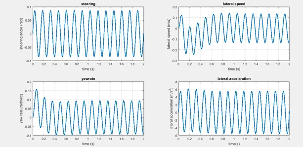 FWD sine plot
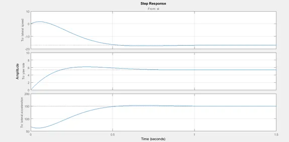 FWD step plot
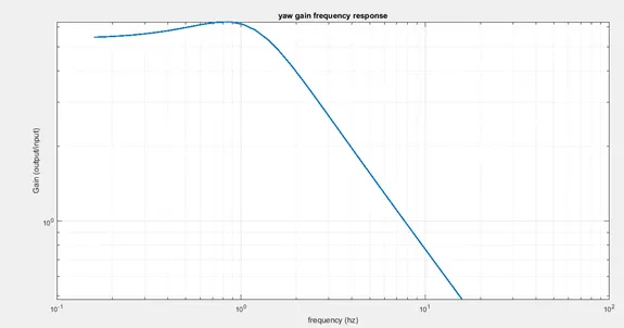 FWD Yaw gain frequency plot
FWD Correlation between different plots:
-correlation at 7 hz:
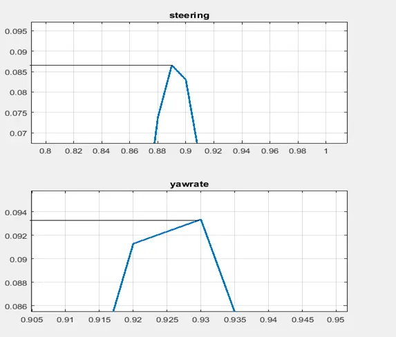
Gain =output/input=0.0935/0.0855=1.093
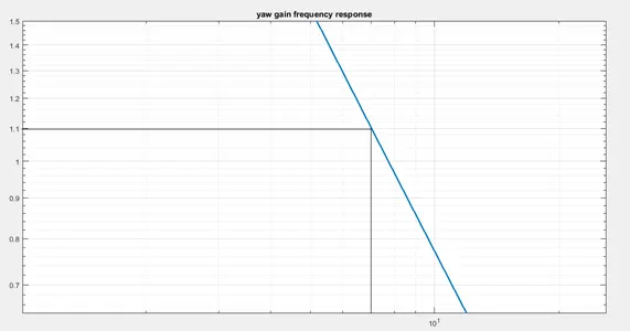
Which is the same in the yaw gain frequency plot
Steady state gain corellation:


Steady state yaw gain means the gain of the system as t tends to infinity or at very low frequency,so here in the step response we find that it reaches steady state output value of 5.4 for a unity step input ,so the steady state gain is 5.4
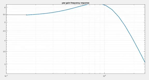
Which is the same for the yaw gain frequency plot
Rise time corellation:

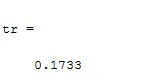
There is a deviation between rise time analytical calculation and calculating it automatically using step info function in matlab but it is acceptable
Results:
YB=Cf+Cr=-1.125*10^5
YR=(a*Cf-b*Cr)/u=6.1172*10^4
YS=-Cf=6.1172*10^4
NB=a*Cf-b*Cr=2.9615*10^4
NR=(((a^2)*Cf)+((b^2)*Cr))/u=-6.7344*10^3
NS=-a*Cf=5.4444*10^4
Wn=sqrt(((YB*NR)+(NB*m*u)-(YR*NB))/(m*u*jz))=7.1912 rad/s
Theta=abs(-((NR/jz)+(YB/(m*u)))*(1/(2*Wn)))=0.72245
Wd=Wn*sqrt(1-(Theta)^2)=4.9564 rad/s
tr=((m*u*NS)/((YS*NB)-(YB*NS)))=0.1733 s
F1 CODE:
clear all
close all
clc
l = 2.901696 ; % Wheelbase (m)
a = 1.740408; % cg to front axle (m)
b = l-a; % cg to rear axle (m)
m = 779.725284; % Mass (kg)
jz = 865 ; % moment of inertia (kg-m^2)
cf = 276803.935; % front cornering stiffness (N/rad)
cr = 429733.794; % rear cornering stiffness (N/rad)
u = 350/3.6; % m/s
A=[-(cf+cr)/(m*u),(((b*cr)-(a*cf))/(m*u))-u;((b*cr)-(a*cf))/(jz*u),-((((a^2)*cf)+((b^2)*cr))/(jz*u))]
B=[cf/m;(a*cf)/jz]
c1=[1,0] %lateral speed
d1=0
c2=[0,1] % yaw rate
d2=0
c3=A(1,:)+u*[0,1] %lateral acceleration
d3=B(1)
t=[0:0.01:2]
st=(pi/180)*5*sin(2*pi*7*t)
C=[c1;c2;c3]
D=[d1;d2;d3]
sys=ss(A,B,C,D)
Y=lsim(sys,st,t)
sys.Inputname={'st'}
sys.Outputname={'lateral speed','yaw rate','lateral acceleration'}
[mag1,phase1,omega1] = bode(sys({'yaw rate'},{'st'}))
for i=1:length(mag1)
magnitude1(i)=mag1(1,1,i)
i=i+1
end
figure(1)
loglog(omega1/(2*pi),magnitude1,'linewidth',2)
title('yaw gain frequency response')
grid on
grid on
figure(2)
subplot(2,2,1)
plot(t,st,'linewidth',2)
title('steering')
grid on
subplot(2,2,2)
plot(t,Y(:,1),'linewidth',2)
title('lateral speed')
grid on
subplot(2,2,3)
plot(t,Y(:,2),'linewidth',2)
title('yawrate')
grid on
subplot(2,2,4)
plot(t,Y(:,3),'linewidth',2)
title('lateral accelaration')
grid on
figure(3)
step(sys)
grid on
S=stepinfo(sys)
[wn theta]=damp(sys)
Cf = -276803.935; % front cornering stiffness (N/rad)
Cr = -429733.794;
YB=Cf+Cr
YR=(a*Cf-b*Cr)/u
YS=-Cf
NB=a*Cf-b*Cr
NR=(((a^2)*Cf)+((b^2)*Cr))/u
NS=-a*Cf
Wn=sqrt(abs(((YB*NR)+(NB*m*u)-(YR*NB))/(m*u*jz)))
Theta=abs(-((NR/jz)+(YB/(m*u)))*(1/(2*Wn)))
Wd=Wn*sqrt(1-(Theta)^2)
tr=abs((m*u*NS)/((YS*NB)-(YB*NS)))
Steps:
-first input is declared
-then A matrix is inputted using A=[-(cf+cr)/(m*u),(((b*cr)-(a*cf))/(m*u))-u;((b*cr)-(a*cf))/(jz*u),-((((a^2)*cf)+((b^2)*cr))/(jz*u))]
-then b matrix is inputted using: B=[cf/m;(a*cf)/jz]
-then output for the lateral speed specified using c1 and d2 matrix:
c1=[1,0]
d1=0
-then output for yaw rate is specified using c2 and d2 matrix:
c2=[0,1]
d2=0
-then output for lateral acceleration is specified usingc3 and d3 matrix: c3=A(1,:)+u*[0,1]
d3=B(1)
where A(1,:) means the first row in A matrix with all the column and b(1) means the first element in the b matrix
-then time array is form from 0 and 2 with 0.01 step in between
-then sinusoidal steering input function is declared using: st=(pi/180)*5*sin(2*pi*7*t)
-then all the outputs are combined in and c and d column array
-then a state space system is formed from the A,B,C,D matrix
-then linear simulation is performed on the system using lsim command to simulate the system dynamic behavior with time with the steering function and time as input, this linear simulation will be performed on all the outputs which will simulate them with respect to time with the steering function as input
-then the inputs and outputs of the state space system are named using input and output channels naming commands: sys.input name and sys.output name
-then bode command is used to store the gain magnitude and phase and frequency in an array
-then in order to turn the 3-dimensional matrix of the magnitude into one dimension, a for loop is used to store the magnitude value from the 3 dimensional matrix into one dimensional array
-then it can be plotted using log scale with frequency ,and the frequency is changed to hz
-then subplot command with 2 rows and 2 columns with first element is the sinusoidal output for steering with time
-then subplot command with 2 rows and 2 columns with second element is the sinusoidal output for lateral speed which is plotted using the first column of y array with all the rows
-then subplot command with 2 rows and 2 columns with third element is the sinusoidal output for lateral speed which is plotted using the second column of y array with all the rows
-then subplot command with 2 rows and 2 columns with fourth element is the sinusoidal output for lateral speed which is plotted using the third column of y array with all the rows
-then step response of the system was plotted using step command
-then all the step response parameters are stores in an array s using step info command, this will be used for correlation with analytical calculations
-then using damp command matlab automatically calculates the natural frequency and the damping ratio of the system and stores them in an array
-calculating the values was done using:
-first yb coefficient is calculated using:
YB=Cf+Cr
-Then yr coefficient is calculated using
YR=(a*Cf-b*Cr)/u
-Then ys coefficient is calculated using
YS=-Cf
-Then nb coefficient is calculated using
NB=a*Cf-b*Cr
-Then nr coefficient is calculated using
NR=(((a^2)*Cf)+((b^2)*Cr))/u
Then ns coefficient is calculated using
NS=-a*Cf
Then wn is calculated using
Wn=sqrt(((YB*NR)+(NB*m*u)-(YR*NB))/(m*u*jz))
Then damping ratio theta is calculated using
Theta=abs(-((NR/jz)+(YB/(m*u)))*(1/(2*Wn)))
Then damped natural frequency is calculated using
Wd=Wn*sqrt(1-(Theta)^2)
Then rising time is calculated using
tr=((m*u*NS)/((YS*NB)-(YB*NS)))
plots:
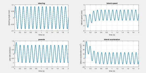 F1 sine plot
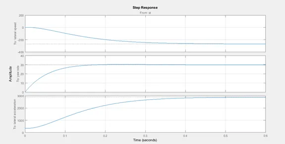 F1 step plot
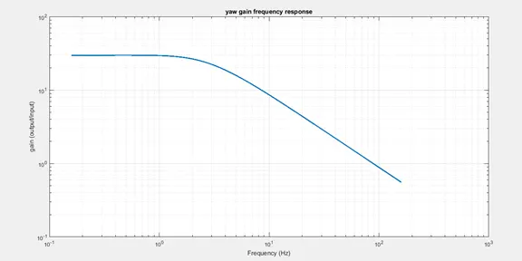 F1 Yaw gain frequency plot
FWD Correlation between different plots:
-correlation at 7 hz:
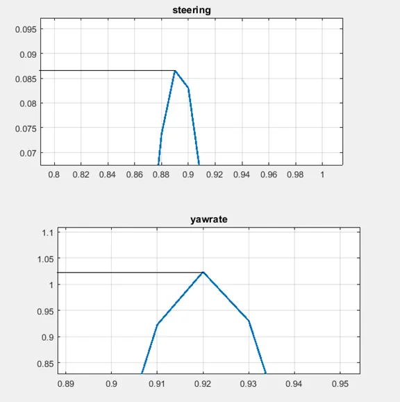
Gain =1.03/0.0855=12.04
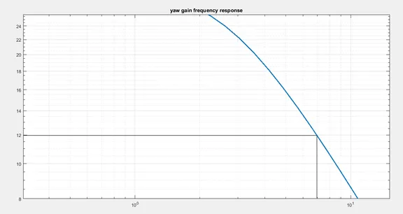
Which is the same in the yaw gain frequency plot
Steady state gain corellation:

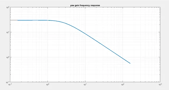
The steady state gain of 30 is found in the time plot as well as the frequency plot
Rise time corellation:

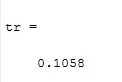
There is a small deviation between rise time analytical calculation and calculating it automatically using step info function in matlab but it is acceptable
Results:
YB=Cf+Cr=-7.0654*10^5
YR=(a*Cf-b*Cr)/u=177.87
YS=-Cf=2.7680*10^5
NB=a*Cf-b*Cr=1.7293*10^4
NR=(((a^2)*Cf)+((b^2)*Cr))/u=-1.4585*10^4
NS=-a*Cf=4.8175*10^5
Wn=sqrt(((YB*NR)+(NB*m*u)-(YR*NB))/(m*u*jz))=13.3077 rad/s
Theta=abs(-((NR/jz)+(YB/(m*u)))*(1/(2*Wn)))=0.9837
Wd=Wn*sqrt(1-(Theta)^2)=2.3934 rad/s
tr=((m*u*NS)/((YS*NB)-(YB*NS)))=0.1058 s
Files:
FWD file:
https://drive.google.com/file/d/1Psl9G6WXVIgvECcwe5qRpBpr3XeQTQ-z/view?usp=sharing
F1 file:
https://drive.google.com/file/d/1Dbgr0ELs50aalorqRDjhnWFIAVHkMr2q/view?usp=sharing