vehicle dynamics week 10b

Question:

1. Plot showing ISO classification for roads A through H (Use higher end of range for degree of roughness) (10 points)
2. Plot showing the PSD profile (10 points)
3. Overlay of PSD profile on ISO classification and determination of road quality (5 points)
4. Error free Octave code (5 points)

Answer:

Matlab code:

clear all

close all

clc

freq = [0.004

0.005

0.006

0.007

0.008

0.009

0.010

0.012

0.017

0.020

0.024

0.028

0.043

0.055

0.063

0.068

0.071

0.080

0.083

0.089

0.090

0.098

0.105

0.115

0.128

0.135

0.145

0.150

0.154

0.160

0.165

0.166

0.167

0.175

0.180

0.185

0.188

0.190

0.190

0.205

0.210

0.215

0.220

0.235

0.250

0.255

0.275

0.280

0.283

0.285

0.300

0.310

0.320

0.330

0.340

0.350

0.353

0.355

0.360

0.370

0.375

0.380

0.385

0.395

0.410

0.420

0.425

0.430

0.435

0.438

0.440

0.460

0.463

0.465

0.480

0.485

0.486

0.490

0.500

0.510

0.540

0.545

0.560

0.565

0.575

0.585

0.590

0.595

0.610

0.620

0.630

0.650

0.655

0.660

0.670

0.680

0.685

0.686

0.690

0.695

0.696

0.700

0.705

0.710

0.715

0.720

0.725

0.730

0.740

0.750

0.765

0.780

0.790

0.810

0.815

0.820

0.830

0.850

0.855

0.860

0.870

0.880

0.885

0.890

0.900];

amplitude = [0.006759586

0.013802191

0.012220044

0.012805345

0.010055096

0.008674203

0.009906454

0.013565614

0.038077859

0.039514035

0.039376401

0.029351388

0.011087978

0.007155759

0.004009582

0.005053475

0.005426501

0.002758627

0.003146703

0.004278752

0.003605323

0.001118033

0.004605136

0.001110531

0.001926103

0.000599825

0.000790703

0.00082178

0.001138063

0.000449034

0.000344602

0.000439721

0.000485891

0.000661237

0.000247849

0.000282707

0.000336575

0.000260436

0.000338

0.000334243

0.000339473

0.000258116

0.000296182

0.000286092

0.000377324

0.000235117

0.000158941

0.000351811

0.000475459

0.000269363

0.00013499

0.000410917

0.000243289

0.000183098

0.000224051

0.000614261

0.000355537

0.000239772

0.000288619

0.000268181

0.00037814

0.000279647

0.000210043

0.000159755

0.000224234

9.50236E-05

0.000197943

0.000138383

0.000143463

0.00012055

0.000161674

9.97741E-05

8.9633E-05

0.000122986

0.000172037

0.000102941

0.00012442

9.02789E-05

0.000143594

6.29552E-05

9.28956E-05

0.000144869

0.000181894

0.000119478

0.000128017

0.000154808

0.000109269

0.000107822

9.00107E-05

0.000123476

8.48896E-05

0.000116729

0.000156981

0.000189126

0.000140362

0.000287068

0.000162162

0.000229266

0.000138612

7.98678E-05

0.000149275

7.12492E-05

0.00022861

8.03851E-05

0.000140036

5.64396E-05

9.09341E-05

0.000118502

7.68087E-05

7.41522E-05

0.000101869

4.47478E-05

0.000103792

0.000164574

9.03105E-05

9.00065E-05

0.000148517

0.000169078

8.09882E-05

9.06266E-05

9.01182E-05

6.61969E-05

0.000101917

5.92651E-05

6.81185E-05

];

%% Three frequencies - initial, mid and final

omega(1) = 0.01;

omega(2) = 1/(2*pi);

omega(3)= 10;

%% ISO roughness lines - break points

s_ab(2) = 8e-6;

s_bc(2) = 32e-6;

s_cd(2) = 128e-6;

s_de(2) = 512e-6;

s_ef(2) = 2048e-6;

s_fg(2) = 8192e-6;

s_gh(2) = 32768e-6;

s_ab(1)=s_ab(2)*(omega(1)/omega(2))^-2

s_ab(3)=s_ab(2)*(omega(3)/omega(2))^-1.5

s_bc(1)=s_bc(2)*(omega(1)/omega(2))^-2

s_bc(3)=s_bc(2)*(omega(3)/omega(2))^-1.5

s_cd(1)=s_cd(2)*(omega(1)/omega(2))^-2

s_cd(3)=s_cd(2)*(omega(3)/omega(2))^-1.5

s_de(1)=s_de(2)*(omega(1)/omega(2))^-2

s_de(3)=s_de(2)*(omega(3)/omega(2))^-1.5

s_ef(1)=s_ef(2)*(omega(1)/omega(2))^-2

s_ef(3)=s_ef(2)*(omega(3)/omega(2))^-1.5

s_fg(1)=s_fg(2)*(omega(1)/omega(2))^-2

s_fg(3)=s_fg(2)*(omega(3)/omega(2))^-1.5

s_gh(1)=s_gh(2)*(omega(1)/omega(2))^-2

s_gh(3)=s_gh(2)*(omega(3)/omega(2))^-1.5

figure(1)

loglog(omega,s_ab)

hold on

loglog(omega,s_bc)

hold on

loglog(omega,s_cd)

hold on

loglog(omega,s_de)

hold on

loglog(omega,s_ef)

hold on

loglog(omega,s_fg)

hold on

loglog(omega,s_gh)

hold on

freq_n = freq./0.3048;

amplitude_n = amplitude.*(0.3048).^3.*(2*pi)

figure(2)

loglog(freq_n,amplitude_n)

figure(3)

loglog(omega,s_ab)

hold on

loglog(omega,s_bc)

hold on

loglog(omega,s_cd)

hold on

loglog(omega,s_de)

hold on

loglog(omega,s_ef)

hold on

loglog(omega,s_fg)

hold on

loglog(omega,s_gh)

hold on

loglog(freq_n,amplitude_n)

hold on

delta(125)=freq_n(125)-freq_n(124)

for i=1:124

delta(i)=(freq_n(i+1)-freq_n(i))

end

for j =1:500

x(j)=j

total(j)=0

for i=1:125

z(i)=sqrt(amplitude_n(i)*2*delta(i))

total(j)=total(j)+z(i)*sin(freq_n(i)*x(j)*2*pi)

end

end

figure(4)

plot(x,total)

steps:

-frequency is inputted

-then the three frequencies :initial ,mid,final that will be on the x -axis are inputted

-then the middle break points on the y -axis for all the iso roughness lines are inputted

-then the first point on the iso lines is computed from the middle point and frequency using:

s(1)=s(2)*(omega(1)/omega(2))^-2

where s(2) is the middle point and s(1) is the initial point

-then the final point is calculated using: s(3)=s(2)*(omega(3)/omega(2))^-1.5

-then the lines are plotted using log scale with the initial omega point on the x-axis and lines values on the y-axis

-then inputted frequency is converted from cycle/ft to cycle/m

- then amplitude is converted ft^3/rad to m^3/cycle

-then the road profile is plotted using the convered frequency and amplitude using log scale

-then the overlay between road profile and iso lines is plotted on the same plot using log scale

Extra work:

-inorder to get the the space plot for the road profile with height and distance on the y and x-axis, we will need to perform numerical integration

PSD=Zn /delta omega (or 2 delta omega as it should be given)

-so Zn=sqrt amplitude of the psd *2 delta omega

-inorder to compute that the last point the delta is calculated

-then for loop with a counter = number of elements in the frequency array -1 is constructed

With each element=next element-current element

-Then Zn=sqrt amplitude of the psd *2 delta omega

-since temporal frequency=1/L

-so the result is summed to zn *sint(2*pi*x*frequency )

-this is done 124 times to get y representative of a single x point

-then this process is done 500 times to get the full plot (all x points)

-by this method we got the area under the curve which allows us to plot the space plot of the road with height and distance on the y and x axis

plots:

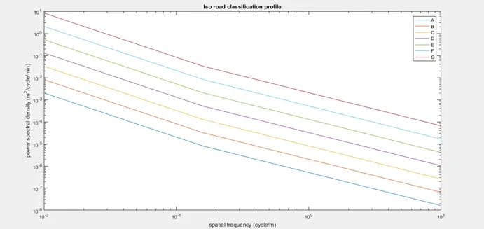Iso lines plot

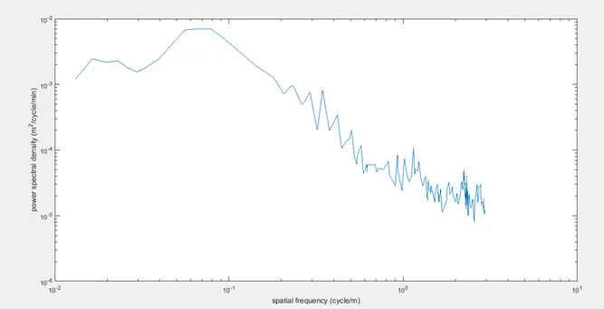Road profile Psd plot

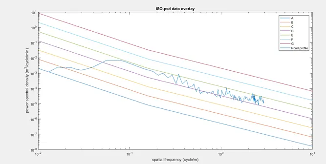Overlay of Iso lines and road profile Psd

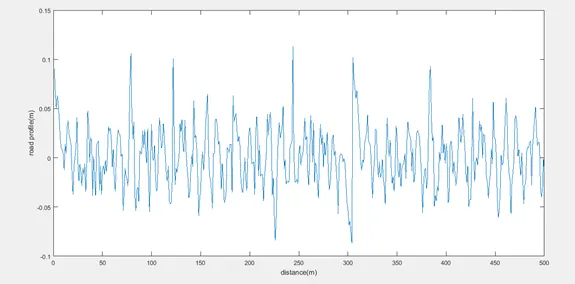space road profile plot (Extra)

conclusion:

This road is E-type road

files:

https://drive.google.com/file/d/1hUUt-2qDnsYst4X7n7uHi6mhLPBz2Scx/view?usp=sharing