A study on the effect of time-step on the stability of the implicit and explicit schemes using MATLAB
OBJECTIVES:
- To study the effect of time step on the stability of the solution for implicit and explicit schemes
- To discuss the CFL number and its effect on the stability of the solution. Also, to plot the unstable solution.
THEORY:
Courant-Friedrichs-Lewy (CFL) condition:
In order to converge explicit and semi-implicit schemes, the time step size needs to be carefully selected, otherwise, the simulation might lead to non-physical results or diverge altogether. The stability requirements of time-integration schemes can be defined using the Courant-Friedrichs-Lewy (CFL) condition. In 2D heat conduction. it can be expressed as -
CFLx + CFLy ≤ 0.5
Transient (Explicit):
For the explicit scheme, the 2D heat conduction can be written as-
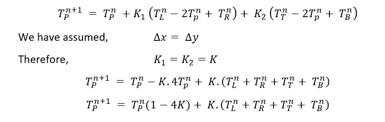
For stability, the coefficient on Tp must be non-negative i.e.
1-4k ≥ 0
K ≤ 0.25
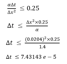
The above equation gives the stability requirement for the solution to be stable. This is because in the explicit approach, for a given Δx, the allowed value of Δt is not independent, and must be small enough to satisfy this criterion. If K ≤ 0.25, the error will not grow for subsequent marching steps in t, and therefore the numerical solution will proceed in a stable manner. But if K ≥ 0.25, then the error will progressively become larger and will eventually cause the time marching solution to 'blow up' on the computer i.e. become unstable. This can happen due to such things as numbers going to infinity or taking the square root of a negative number. Therefore,
Transient(Implicit):
These are unconditionally stable and stability can be maintained over much larger values of Δt, meaning that any value of Δt, no matter how large, will yield a stable solution. Therefore, in some cases, even though the implicit approach requires more computations per time step due to its relative complexity, but the fact that considerably fewer time steps are required to cover a given interval of time can ultimately result in a shorter run time on the computer as compared to an explicit approach.
Note: The CFL criterion doesn't come into the picture for the steady-state as there is no time-derivative term.
CODE & RESULTS:
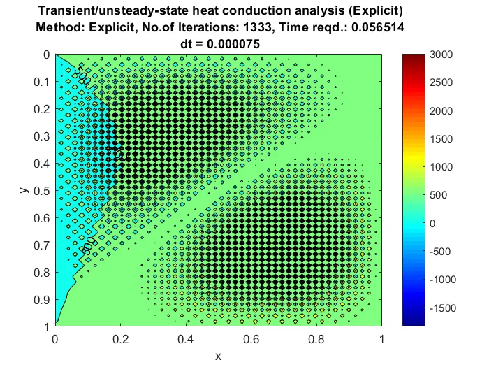
Case1 (Explicit): We observe that when we use a value of Δt ≥ 7.43143e-5, the sum of k1+k2 ≥ 0.5, and therefore, the solution becomes unstable.
CODE:
clear all
close all
clc

L = 1; %Length of the Domain
nx = 50; %Nodes
ny=nx;

x=linspace(0,L,nx);
dx=x(2)-x(1);
y=linspace(0,L,ny);
dy=y(2)-y(1);
t = 0.1;
dt = 7.5e-5; %CFL criteria, dt < 7.43143e-5
nt = t/dt;
alpha = 1.4;
CFL_x= alpha*dt/(dx)^2;
CFL_y= alpha*dt/(dy)^2;
ct = 0;

T=300*ones(nx,ny);
T(:,1)= 400 ; %Left Wall
T(1,:)= 600; %Top Wall
T(:,end)= 800; %Right Wall
T(end,:)= 900; %Bottom Wall

T(1,1)= (400+600)/2 ;
T(1,end)= (600+800)/2 ;
T(end,1)= (400+900)/2 ;
T(end,end)= (900+800)/2 ;

Told = T;
k1 = (alpha*dt)/(dx^2);
k2 = (alpha*dt)/(dy^2);

tic
for k = 1:nt
    for i = 2:nx-1
        for j =2:ny-1
            H = (Told(i-1,j) - 2*Told(i,j) + Told(i+1,j));
            V = (Told(i,j+1) - 2*Told(i,j) + Told(i,j-1));
            T(i,j) = Told(i,j) + k1*H + k2*V;
        end
    end
    Told = T;
    ct = ct+1;
    time = toc;
end
figure(1)
contourf(x,y,T,'ShowText','on');
colorbar
colormap(jet)
xlabel('x');
ylabel('y');
text = sprintf(' Transient/unsteady-state heat conduction analysis (Explicit)n Method: Explicit, No.of Iterations: %d, Time reqd.: %fn dt = %f',ct, time, dt );
title(text);
set(gca,'YDIR','reverse');
OUTPUT:
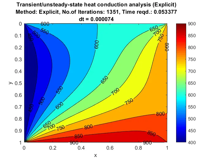
CASE 2 (Explicit): With a value of Δt ≤ 7.43143e-5, the sum of k1+k2 ≤ 0.5. This satisfies the stability criteria and thus the solution is stable.
clear all
close all
clc

L = 1; %Length of the Domain
nx = 50; %Nodes
ny=nx;

x=linspace(0,L,nx);
dx=x(2)-x(1);
y=linspace(0,L,ny);
dy=y(2)-y(1);
t = 0.1;
dt = 7.4e-5; %CFL criteria, dt < 7.43143e-5
nt = t/dt;
alpha = 1.4;
CFL_x= alpha*dt/(dx)^2;
CFL_y= alpha*dt/(dy)^2;
ct = 0;

T=300*ones(nx,ny);
T(:,1)= 400 ; %Left Wall
T(1,:)= 600; %Top Wall
T(:,end)= 800; %Right Wall
T(end,:)= 900; %Bottom Wall

T(1,1)= (400+600)/2 ;
T(1,end)= (600+800)/2 ;
T(end,1)= (400+900)/2 ;
T(end,end)= (900+800)/2 ;

Told = T;
k1 = (alpha*dt)/(dx^2);
k2 = (alpha*dt)/(dy^2);

tic
for k = 1:nt
    for i = 2:nx-1
        for j =2:ny-1
            H = (Told(i-1,j) - 2*Told(i,j) + Told(i+1,j));
            V = (Told(i,j+1) - 2*Told(i,j) + Told(i,j-1));
            T(i,j) = Told(i,j) + k1*H + k2*V;
        end
    end
    Told = T;
    ct = ct+1;
    time = toc;
end
figure(1)
contourf(x,y,T,'ShowText','on');
colorbar
colormap(jet)
xlabel('x');
ylabel('y');
text = sprintf(' Transient/unsteady-state heat conduction analysis (Explicit)n Method: Explicit, No.of Iterations: %d, Time reqd.: %fn dt = %f',ct, time, dt );
title(text);
set(gca,'YDIR','reverse');
OUTPUT:
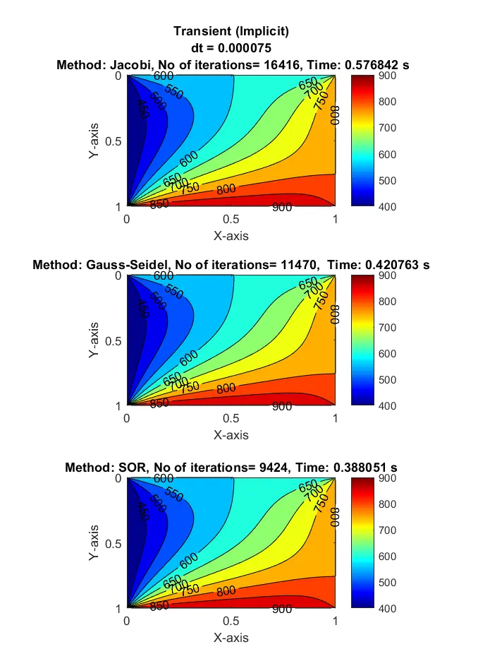
Case 3 (Implicit): We observe that even when we use a value of Δt ≥ 7.43143e-5, the sum of k1+k2 ≥ 0.5, but the solution remains stable.
clear all
close all
clc

L = 1; %Length of the Domain
nx = 50; %Nodes
ny=nx;

x=linspace(0,L,nx);
dx=x(2)-x(1);
y=linspace(0,L,ny);
dy=y(2)-y(1);
t = 0.1;
dt = 7.5e-5; %CFL criteria, dt < 7.43143e-5
nt = t/dt;
omega  = 1.1;
alpha = 1.4;
ct = 0;
ct1 = 0; ct2=0; ct3=0;
error = 9e9;
error1=error;error2=error;error3=error;
tol = 1e-4;

T=300*ones(nx,ny);
T(:,1)= 400 ; %Left Wall
T(1,:)= 600; %Top Wall
T(:,end)= 800; %Right Wall
T(end,:)= 900; %Bottom Wall

T(1,1)= (400+600)/2 ;
T(1,end)= (600+800)/2 ;
T(end,1)= (400+900)/2 ;
T(end,end)= (900+800)/2 ;

T1 = T; T2 = T; T3=T;
Told1 = T1; Told2 = T2; Told3=T;

T_prev1 = T1; T_prev2 = T2;T_prev3 = T3;
k1 = (alpha*dt)/(dx^2);
k2 = (alpha*dt)/(dy^2);

    tic
    for j = 1:nt
        error1 = 9e9;
        while(error1>tol)
            for i = 2:nx-1
                for j =2:ny-1
                    term1_1 = 1/(1+2*k1+2*k2);
                    term2_1 = k1*term1_1;
                    term3_1 = k2*term1_1;
                    H1 = (Told1(i-1,j) + Told1(i+1,j));
                    V1 = (Told1(i,j+1) + Told1(i,j-1));
                    T1(i,j) = (term1_1*(T_prev1(i,j)))+(term2_1*H1)+(term3_1*V1);
                end
            end
            error1 = max(max(abs(Told1-T1)));
            Told1 = T1;
            ct1 = ct1+1;
        end
        T_prev1 = T1;
    end
    time1 = toc;


    tic
    for j = 1:nt
        error2 = 9e9;
        while(error2>tol)
            for i = 2:nx-1
                for j =2:ny-1
                    term1_2 = 1/(1+2*k1+2*k2);
                    term2_2 = k1*term1_2;
                    term3_2 = k2*term1_2;
                    H2 = (T2(i-1,j) + Told2(i+1,j));
                    V2 = (Told2(i,j+1) + T2(i,j-1));
                    T2(i,j) = (term1_2*(T_prev2(i,j)))+(term2_2*H2)+(term3_2*V2);
                end
            end
            error2 = max(max(abs(Told2-T2)));
            Told2 = T2;
            ct2 = ct2+1;
        end
        T_prev2 = T2;
    end
    time2 = toc;

    tic
    for j = 1:nt
        error3 = 9e9;
        while(error3>tol)
            for i = 2:nx-1
                for j =2:ny-1
                    term1_3 = 1/(1+2*k1+2*k2);
                    term2_3 = k1*term1_3;
                    term3_3 = k2*term1_3;
                    H3 = (T3(i-1,j) + Told3(i+1,j));
                    V3 = (Told3(i,j+1) + T3(i,j-1));
                    T3(i,j) = (1-omega)*(Told3(i,j)) + (omega*((term1_3*(T_prev3(i,j)))+(term2_3*H3)+(term3_3*V3)));
                end
            end
            error3 = max(max(abs(Told3-T3)));
            Told3 = T3;
            ct3 = ct3+1;
        end
        T_prev3 = T3;
    end
    time3 = toc;

p1 = [.4 .685 .2 .2];
subplot('Position',p1);
contourf(x,y,T1,'ShowText','on');
colorbar
colormap(jet)
xlabel('X-axis');
ylabel('Y-axis');
xticks([0 0.5 1])
text = sprintf('Transient (Implicit)n dt = %f n Method: Jacobi, No of iterations= %d, Time: %f s', dt, ct1 ,time1);
title(text);
set(gca,'YDIR','reverse');

p2 = [.4 .38 .2 .2];
subplot('Position',p2);
contourf(x,y,T2,'ShowText','on');
colorbar
colormap(jet)
xlabel('X-axis');
ylabel('Y-axis');
xticks([0 0.5 1])
text = sprintf('Method: Gauss-Seidel, No of iterations= %d,  Time: %f s',ct2 ,time2);
title(text);
set(gca,'YDIR','reverse');

p3 = [.4 .07 .2 .2];
subplot('Position',p3)
contourf(x,y,T3,'ShowText','on');
colorbar
colormap(jet)
xlabel('X-axis');
ylabel('Y-axis');
xticks([0 0.5 1])
text = sprintf('Method: SOR, No of iterations= %d, Time: %f s',ct3 ,time3);
title(text);
set(gca,'YDIR','reverse');
OUTPUT: