Surface preparation and Boundary Flagging of a Port Fuel Injected Internal combustion engine
AIM:
1) To flag the boundaries for a PFI internal combustion engine.
2) To prepare the surface of the PFI engine so that the geometry does not have any issues while running the simulation.
3) To run a no hydro simulation and create an animation for it.
INTRODUCTION AND THEORY:
PFI Engine:
Port fuel injected internal combustion engine or PFI IC Engine is a type of IC engine where the fuel is injected into the intake port so that it is mixed with the incoming air. The fuel injectors in PFI engines are typically mounted in the intake manifold and the air/fuel mixture is pulled into the cylinder head as the intake valve opens.
Boundary Flagging in Converge:
Boundary flagging as the name suggests is to designate the boundaries of a geometry. Boundaries are the collection of triangles in a geometry in converge. By flagging boundaries the geometry manipulation becomes easier and we can assign different conditions at each boundary to apply the actual conditions in a specific part of the geometry where by defining how that particular part should behave during the simulation. We can perfrm a lot of other operations like, if we want to view inside a particular section of the geometry, one of the easiest ways is that we can hide that particular geometry if the requried outcome can be obtained by doing so.
There are many methods to flag boundaries that converge offers. The methods which are used in setting up this case are explained briefly below:
1) Any: In this method we select the triangles at a time and when the selection is complete, we set that selection as a boundary. This method is time consuming and tedious when the boundary to be flagged has a large number of triangles.
2) Angle: This method uses the angle between the normals of triangles when selecting the triangles for a particular boundary. There is an option for setting up the maximum angle between the normals of the triangles (which are connected to each other) below which all the triangles can be selected at a time with one single selection of a triangle. For example, if the maximum angle is set to 10 degrees, then by selecting one triangle, those triangles which are connected immediatly adjacent to that triangle get selected whose angle between the adjacent triangle normal falls below 10 degrees, the maximum angle criteria. Then we can set them as a boundary by just a few clicks. This method is easy and can become more flexible by changing the maximum angle parameter. The maximum value of the maximum angle parameter is 90 degrees and the minimum value is 0 degrees.
3) Boundary: This method of selecting the triangles for boundary flagging is used when a boundary that has already been flagged needs to be reflagged into another boundary or if two or more boundaries are required to form another single boundary.
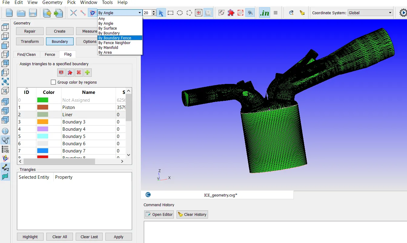
4) Boundary fence: Boundary fence means to create a fence around a set of triangles which are required to form a boundary. A boundary fence is a very useful method of boundary flagging as the fencing can be done for irregular shapes and then can be flagged into a boundary. There are many ways to create a boundary fence. The methods which are used in setting up this case is given below.
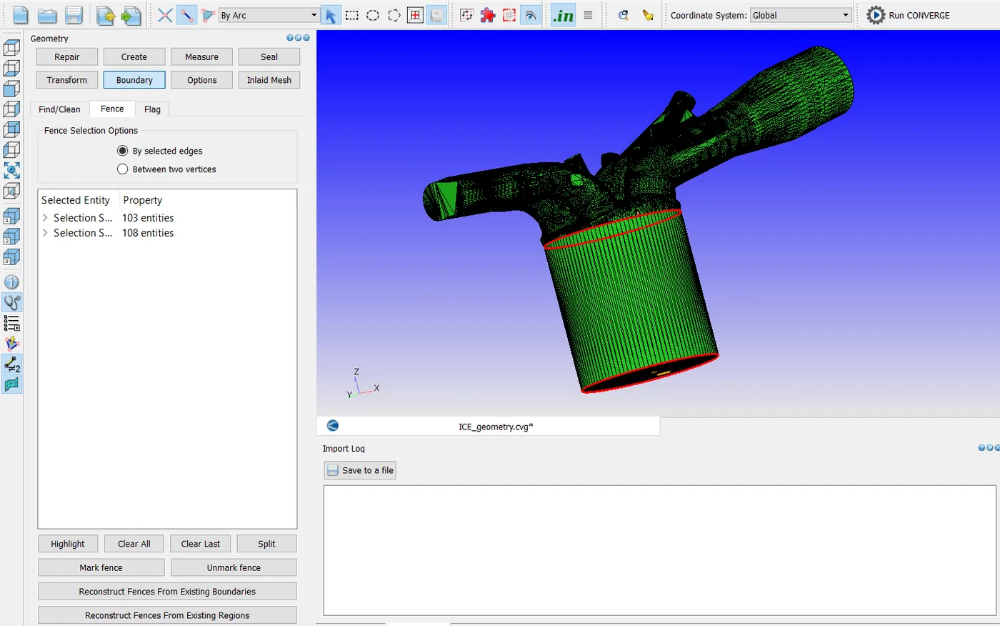
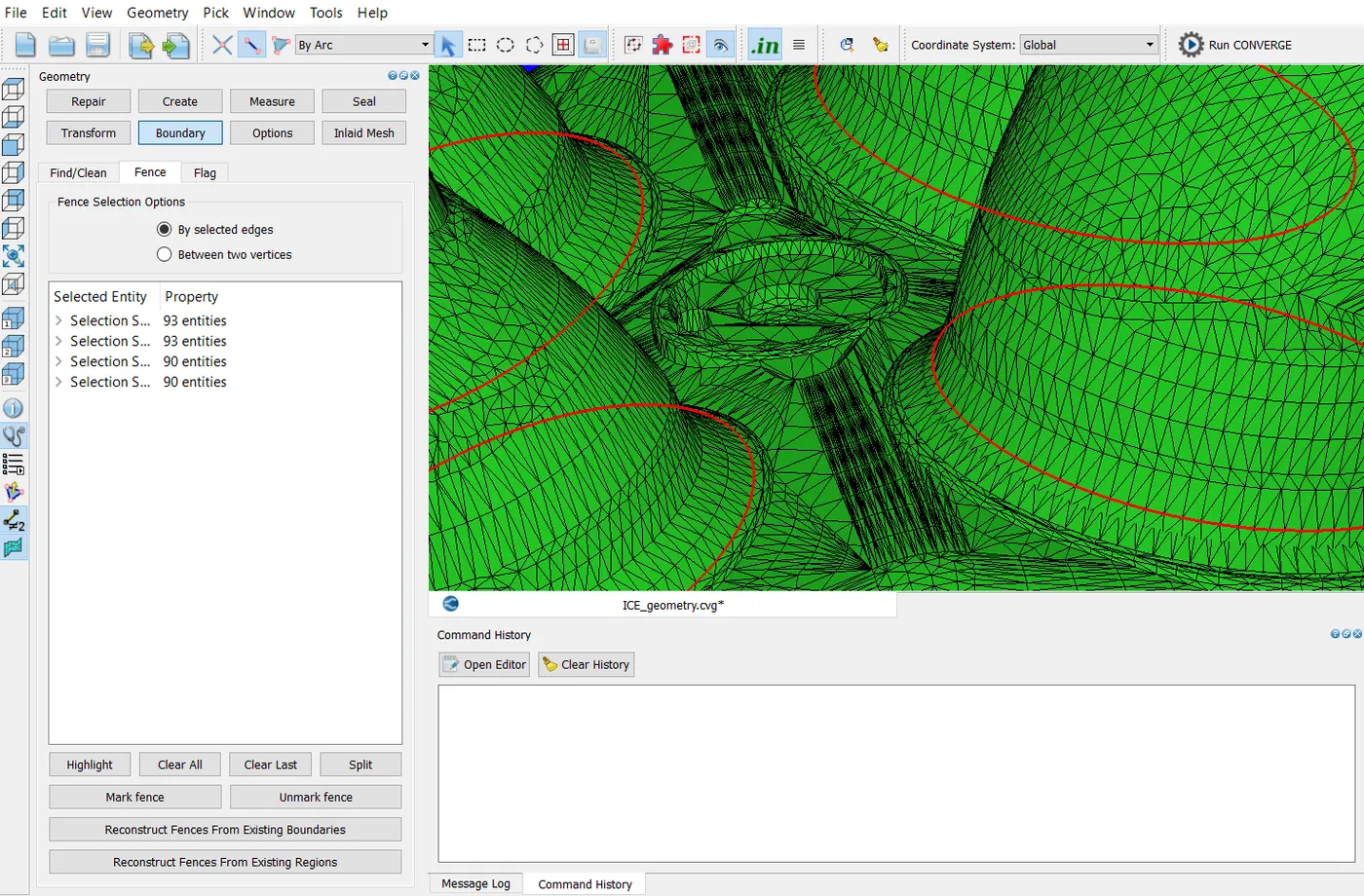
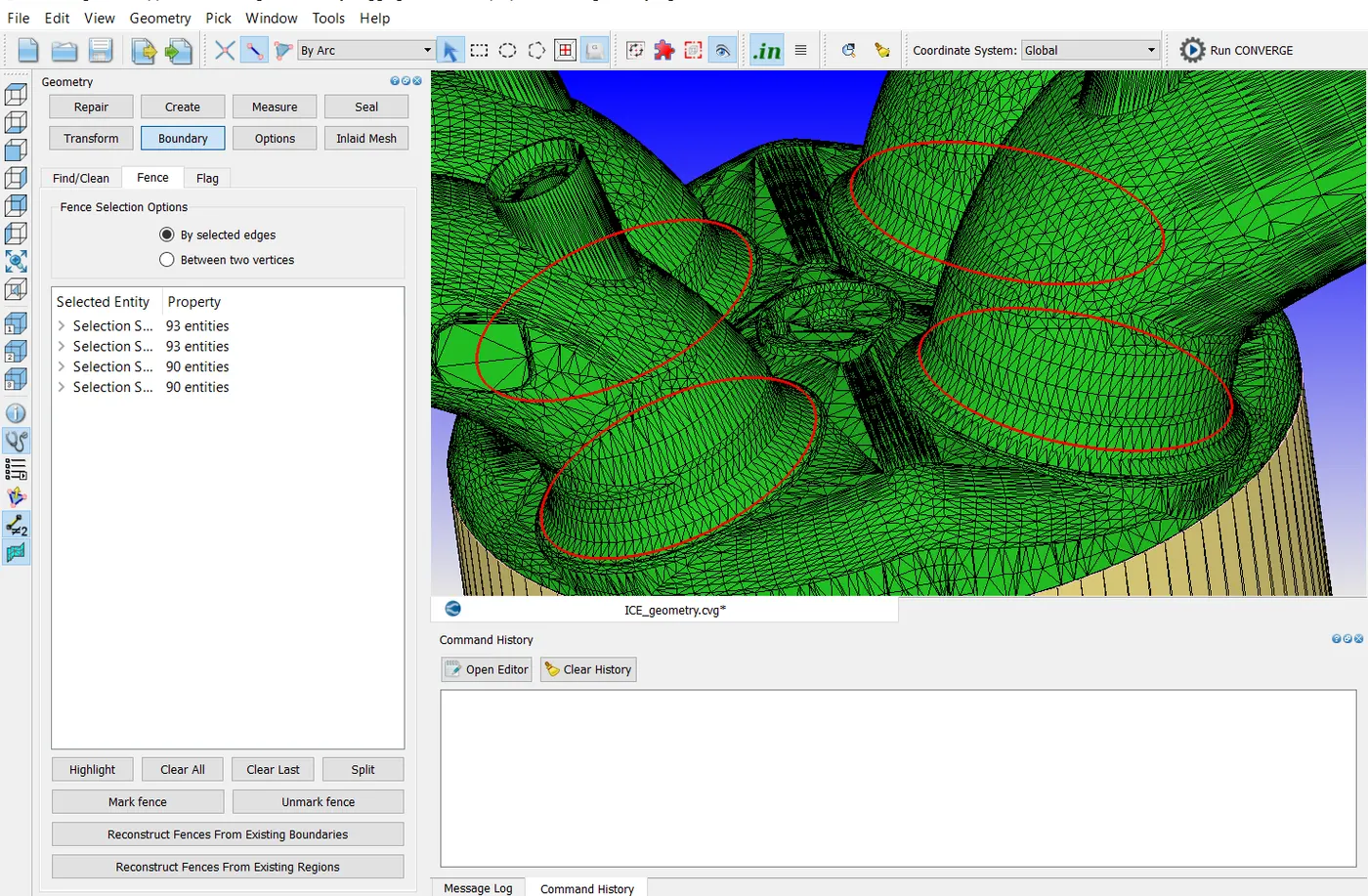
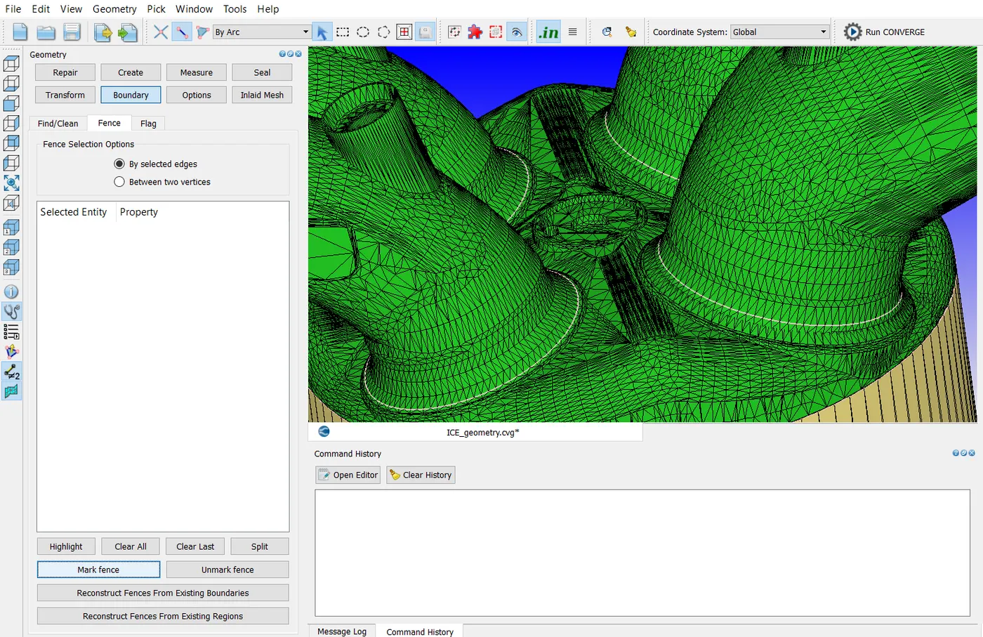
By selected edges and edges selection By arc: In this method, the edges which are required to form a boundary fence are selected by using the arc type selection of edges which selects the edges by seeing if they form an arc together. This method is very useful when we want to make circular boundary fences.
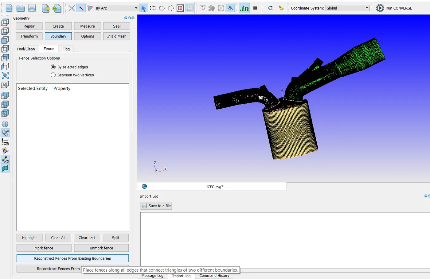
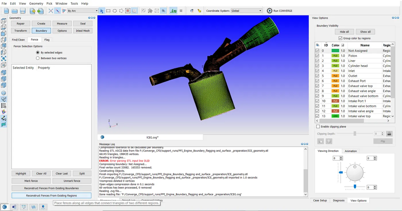
Reconstruct fences from existing boundaries: By clicking this option, boundary fences can be created across each existing boundary. If there is a situation where we are unable to mark a boundary fence and that region is the only region to be fenced and flagged as a bounary then, we can use this method to mark boundary fences from existing boundaries to indirectly construct the boundary fence for the remaining region. This way we can flag this type of boundary.
Surface preparation in converge:
The geometry which is imported from a CAD software is done so by converting it into an stl file. This file format is a triangulated form of the CAD drawing of the geometry which means that the geometry is entirely made up of triangles. Though the geometry which is imported from the CAD softwares is made correctly without any mistakes, the drawing file when converted into an .stl file can get issues which are not accepted in Converge.
This requires some modification and fixing of geometry before setting up a case in converge. This modification of geometry is called "Surface preparation". The first step in preparing the surface is to check for any errors in the surfac ewhich are not allowed in Converge. This is called "Diagnosis". In diagnosis the following are checked for and are also considered as errors in geometry in Converge studio.
1) Intersections
2) Non-Manifold problems
3) Open Edges
4) Normal orientations
1) Intersections: Intersections means when a triangle in a geometry passes through one or more triangles. Threre is a rule in converge that every triangle which is connected to any other triangle must be connected through a commen edge or a common vertex. In case of intersections, as the triangles passes through each other, they are coonected in a way but do not have any edge or vertex in common in that connection.
2) Non-Manifold problems: Non-manifold problems occur when a triangle is connected to more than one triangle having the same edge in common. There is a rule in converge that an edge should be shared by two triangles only. In case of non-manifold problem we have more than two triangles connected to each other through the same common edge. But, in some cases such as in conjugate heat transfer simulation the geometry requirement will be in such a way that certain triangles definitely need to have non-manifold problems but are ignored by converge when this type of case is set up.
3) Open edges: Open edges are those edges which are a part of only one triangle. As Converge requires each edge to be connected two exactly two triangles, being a part of only one triangle is a problem and such a geometry having these edges needs to be momdified before setting up a case in converge.
4) Normal orientations: There is a rule in converge that the direction of normals of each triangle of a geometry should point either inside the fluid domain or outside the fluid domain.Normal orientation problems occur when the direction of normals of one or more triangles does not follow with the rest of the triangles. To study the fluid flow over a geometry all the normals of the triangles must point outside the geometry and while studying the fluied flow inside the geometry the normals of the triangles must point inside the geometry in order to setup the case in Converge.
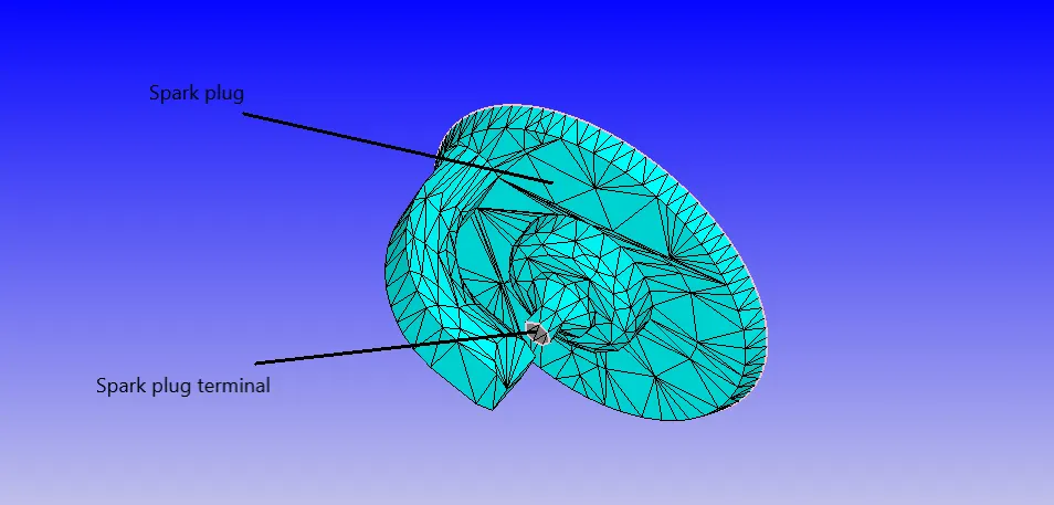
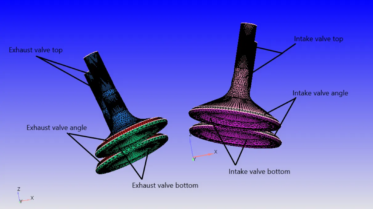
Parts of a typical PFI Engine:
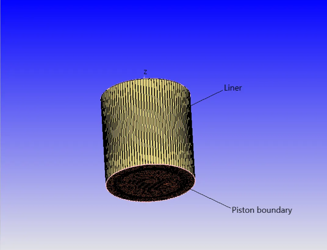
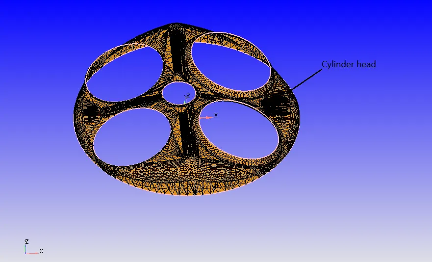
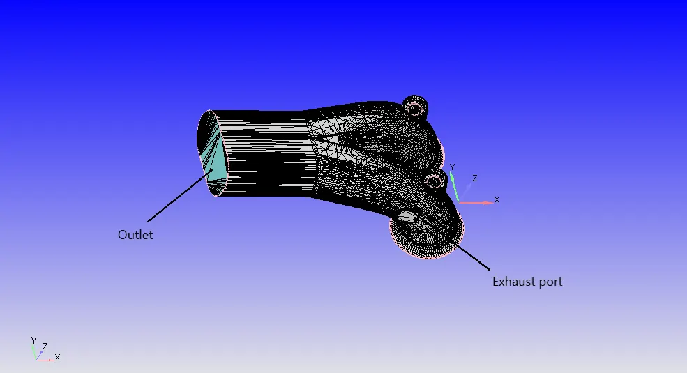
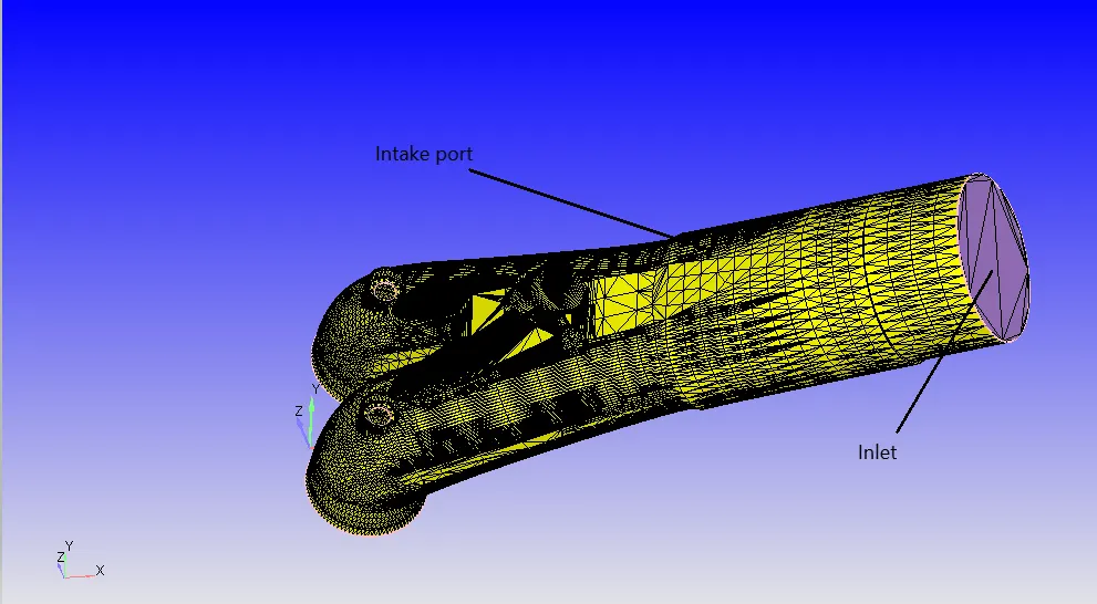
Different parts of a typical PFI engine are labelled in the images shown below:
GEOMETRY OF A PFI ENGINE:
The geometry of a PFI engine is imported as a .stl file. The image of it is shown below.
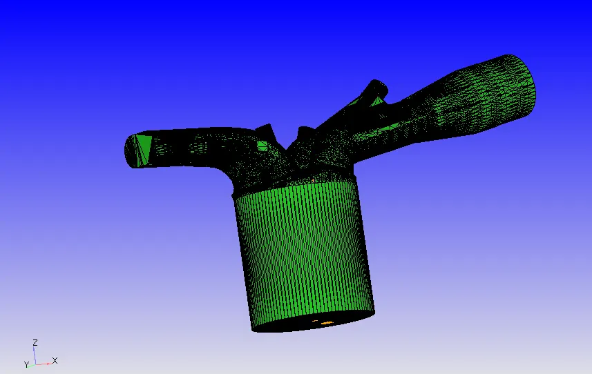
The first step is to assign meaningful boundaries to this geometry which is called boundary flagging.
Boundary Flagging:
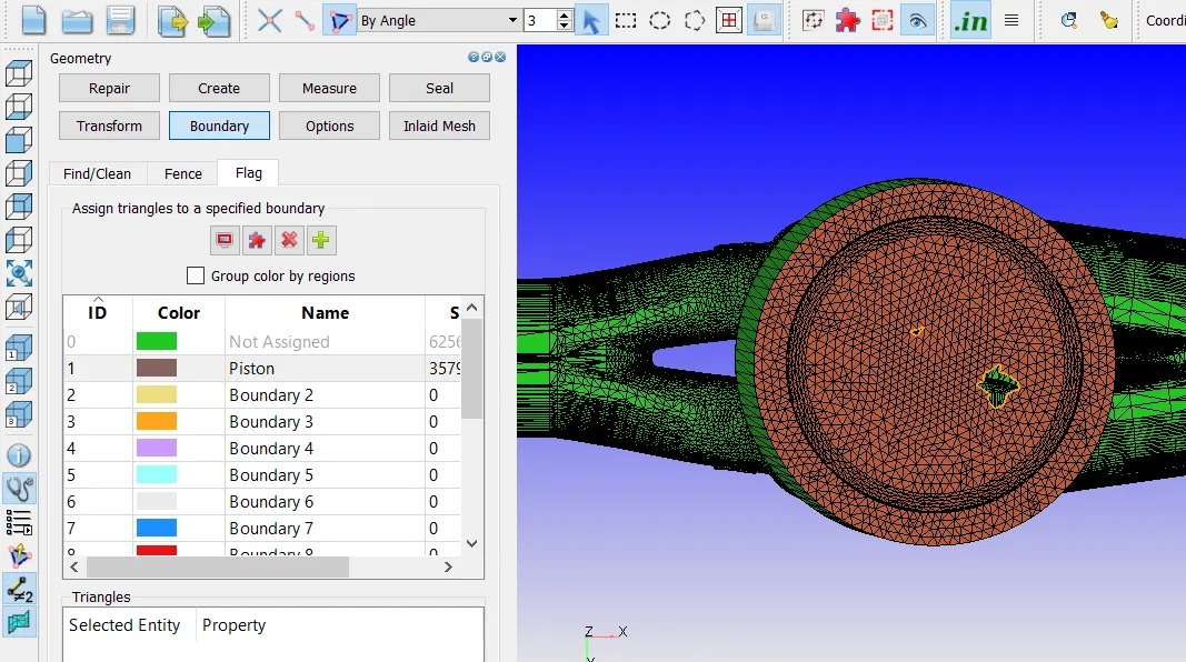
First boundary which is going to be flagged is the piston boundary which is at the bottom of the engine.
We use the angle method to flag the piston boundary.
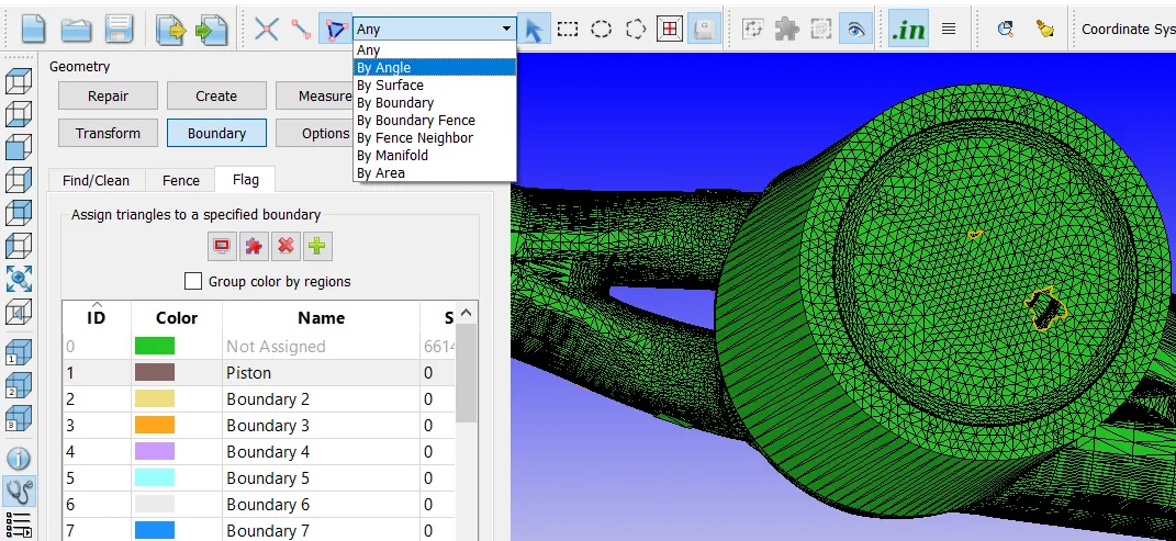
The next boundary to be flagged is the liner. First boundary fences are marked using the method By selected edges and the selection of edges done by using the arc method as shown in the image below.
The boundary fence method is selected and the region between the two boundary fences is selected. This is shown in the two below consecutive images.
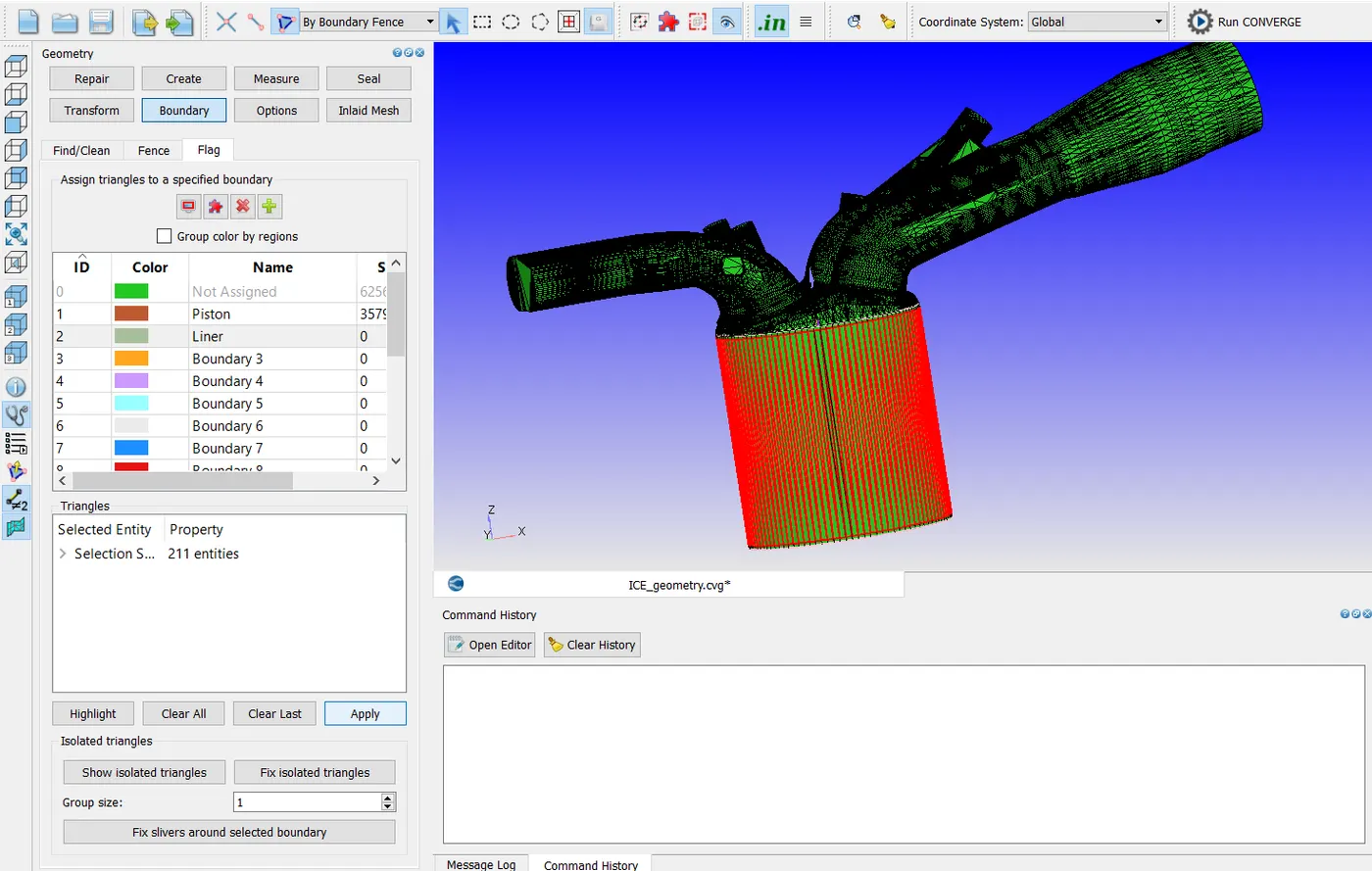
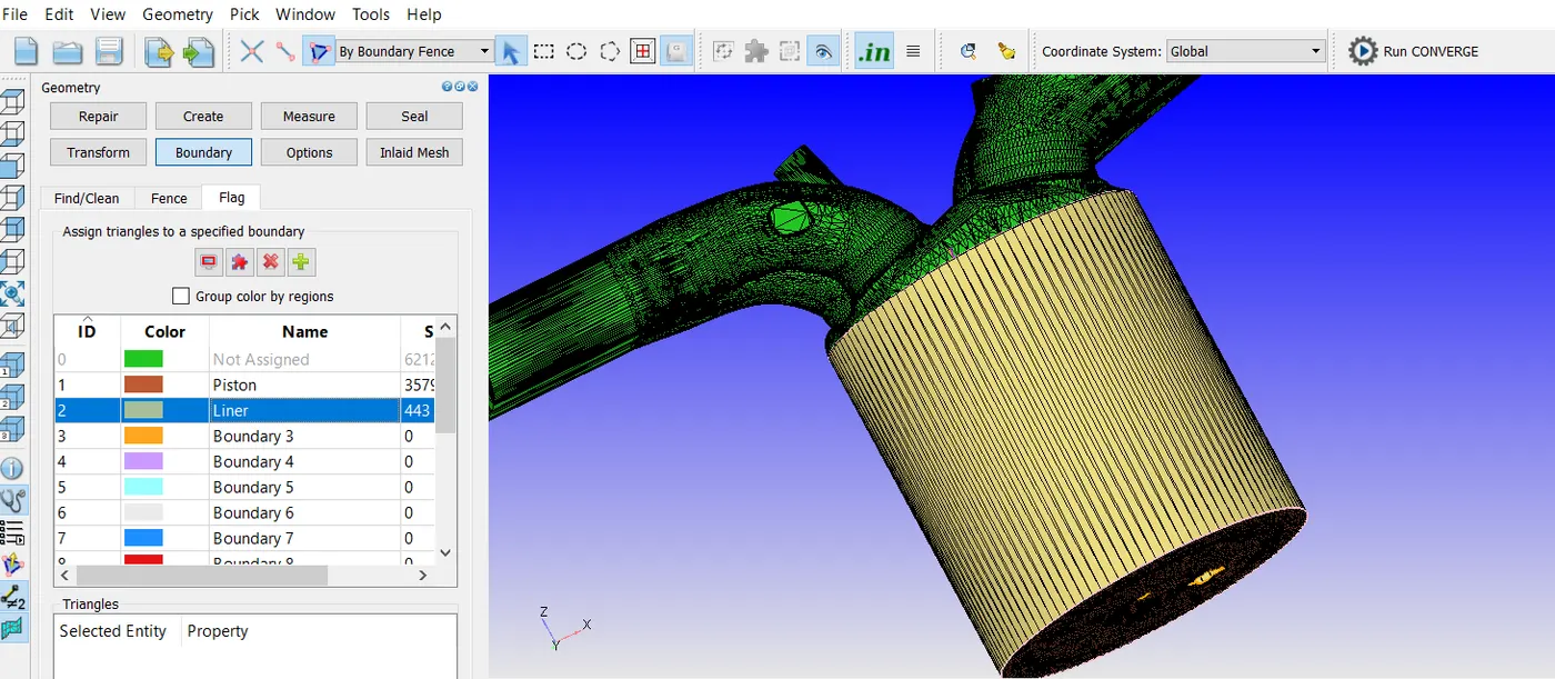
To flag the liner boundary apply option is clicked. The liner boundary is shown in the image below.
Third boundary to be flagged is the cylinder head. The boundary fencing is done using the by arc method under the selected edges as shown in the below three images.
Now, the cylinder head is selected using the boundary fence method to flag as shown in the image below.
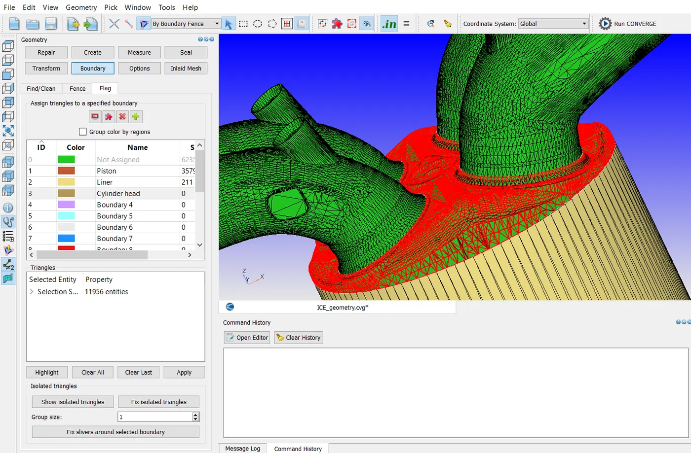
To flag the cylinder head boundary apply option is clicked.
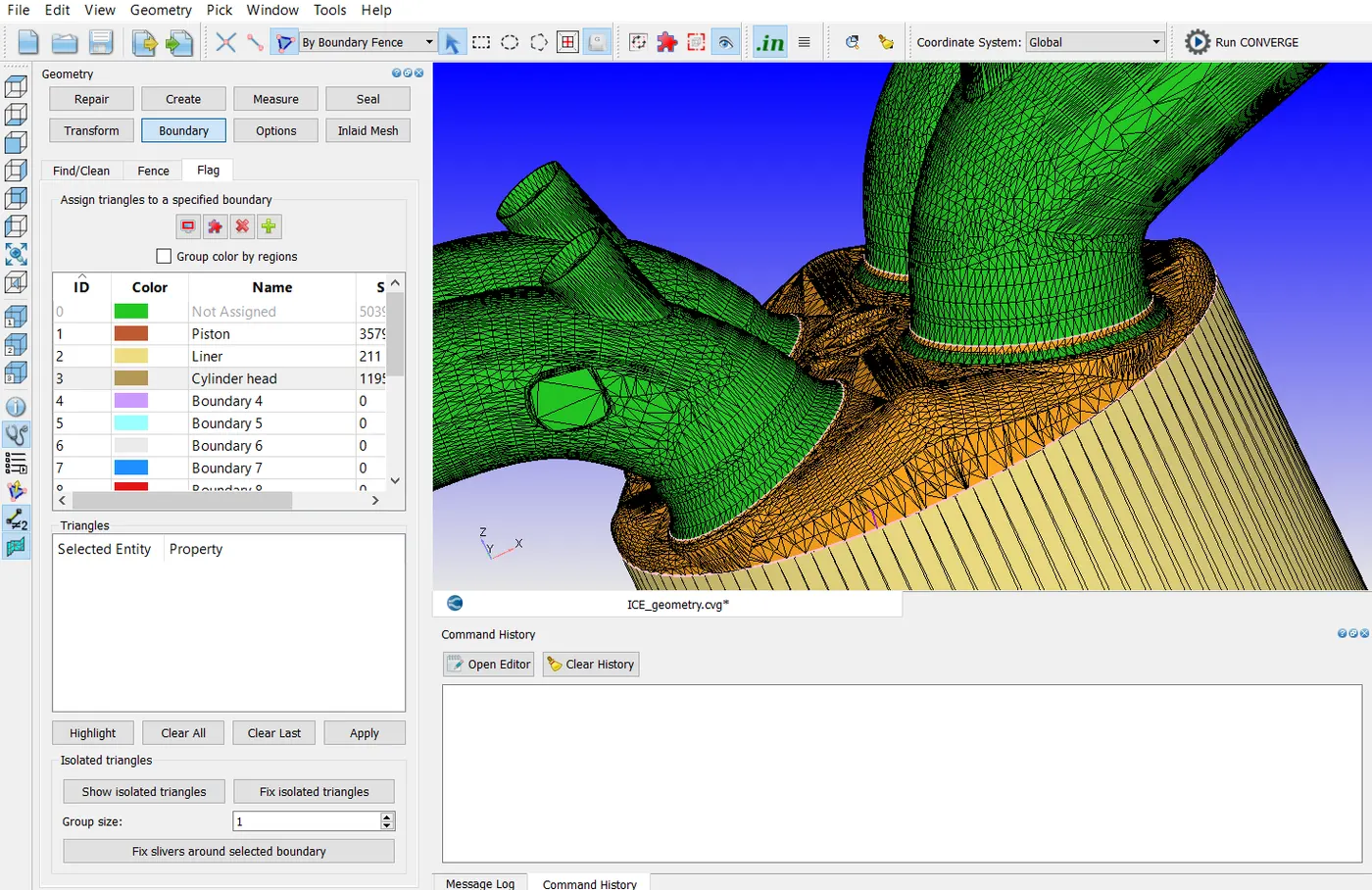
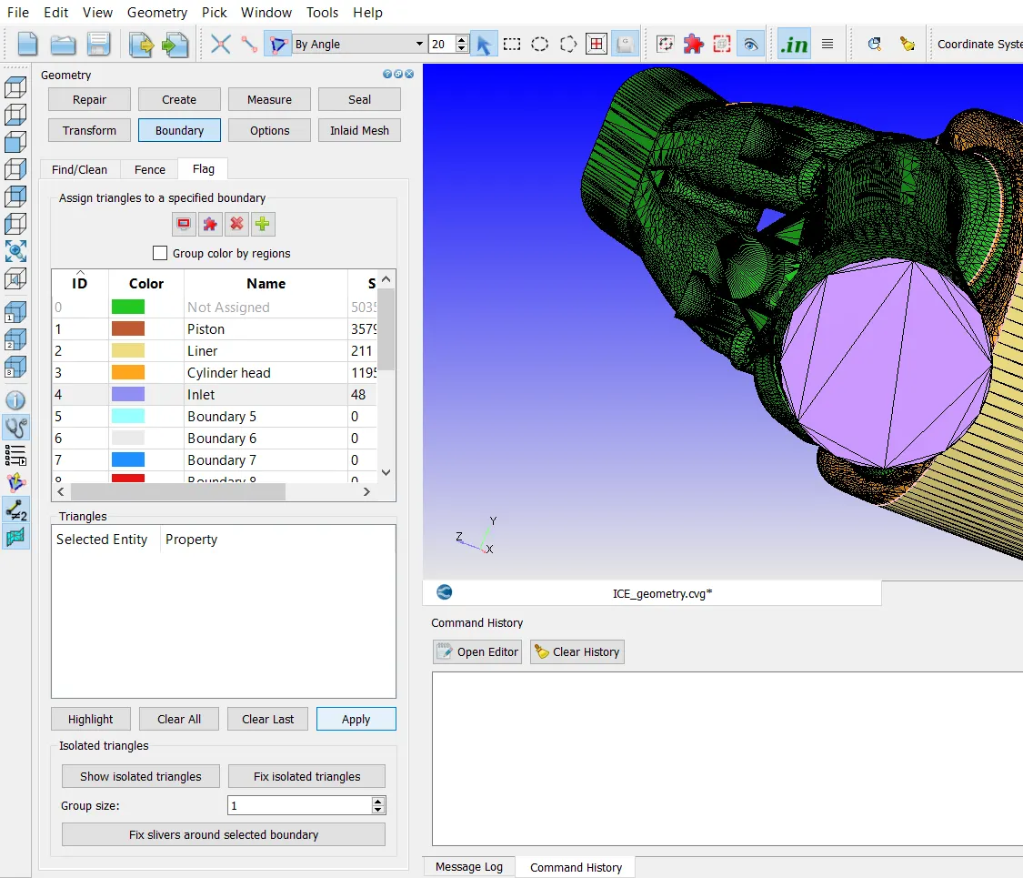
The fourth boundary to be flagged is the inlet boundary. By using the angle method, the inlet boundary is flagged. An image of inlet boundary is shown below.
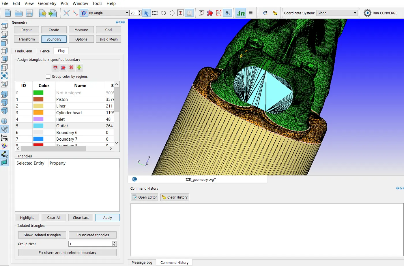
The fifth boundary to be flagged is the outlet boundry. It is flagged by using the angle method. An image of outlet boundary is shown below
The sixth boundary to be flagged is the exhaust port. The exhaust port is selected using the angle method as shown in the image below.
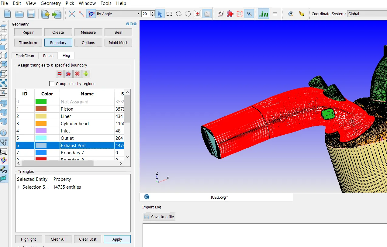
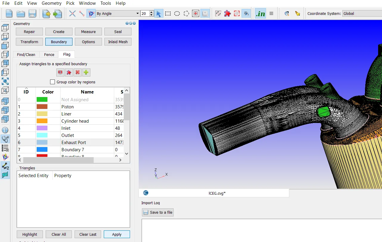
Now, to flag the Exhaust port boundary apply option is clicked. An image of Exhaust port is shown below.
Now, the piston, liner and cylinder head, inlet, outlet and exhaust port boundaries are hidden so that it becomes easier for us to flag the remaining boundaries. A corresponding image is shown below.
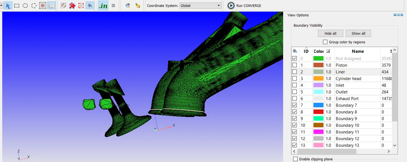
Next boundaries which are to be flagged are Exhaust valve boundaries, namely, exhaust valve top, exhaust valve angle and exhaust valve bottom.
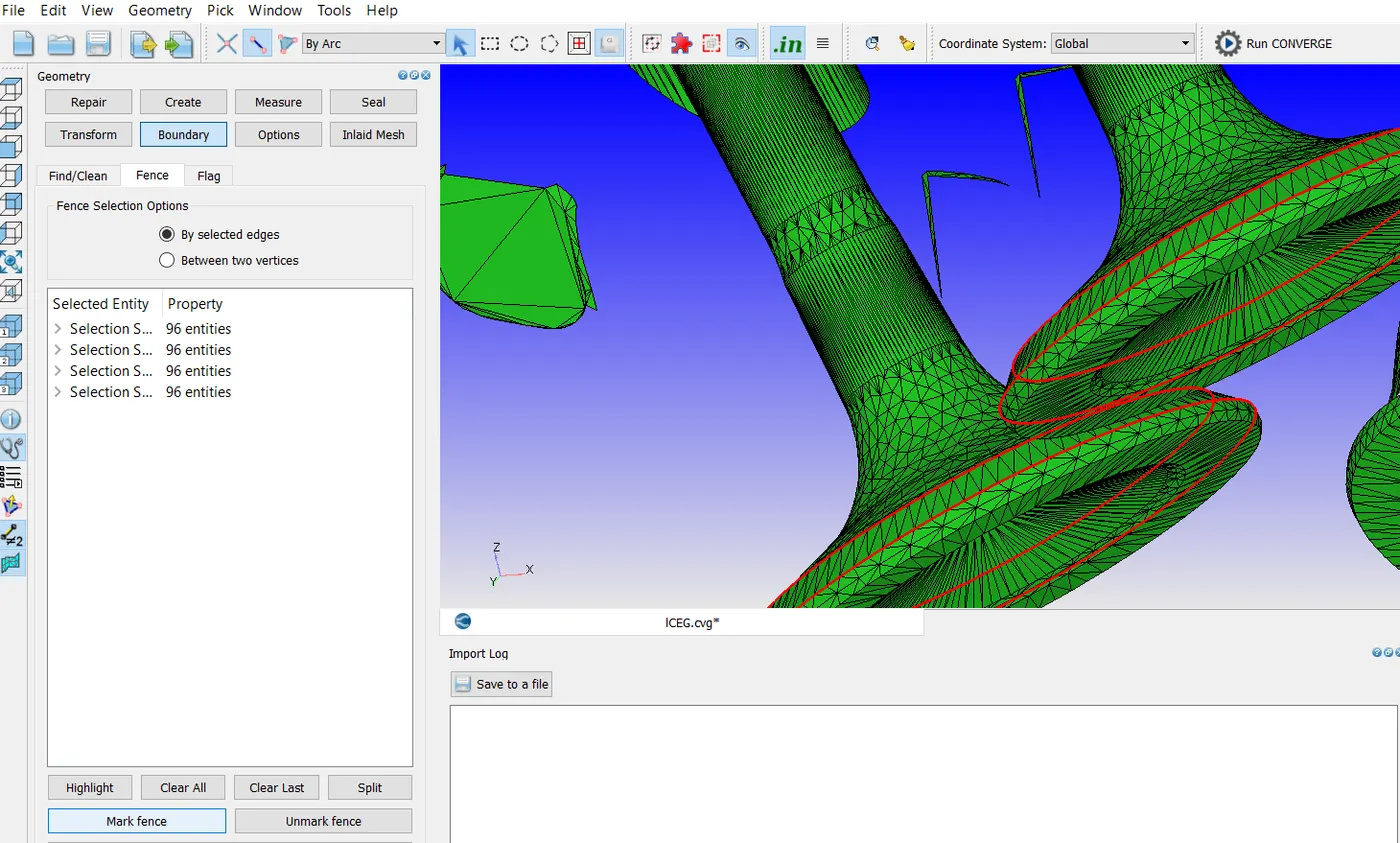
Boundary fences separating the top, angle and bottom exhaust valve boundaries are marked by using the arc method under the selected edges method as shown in the below two images.
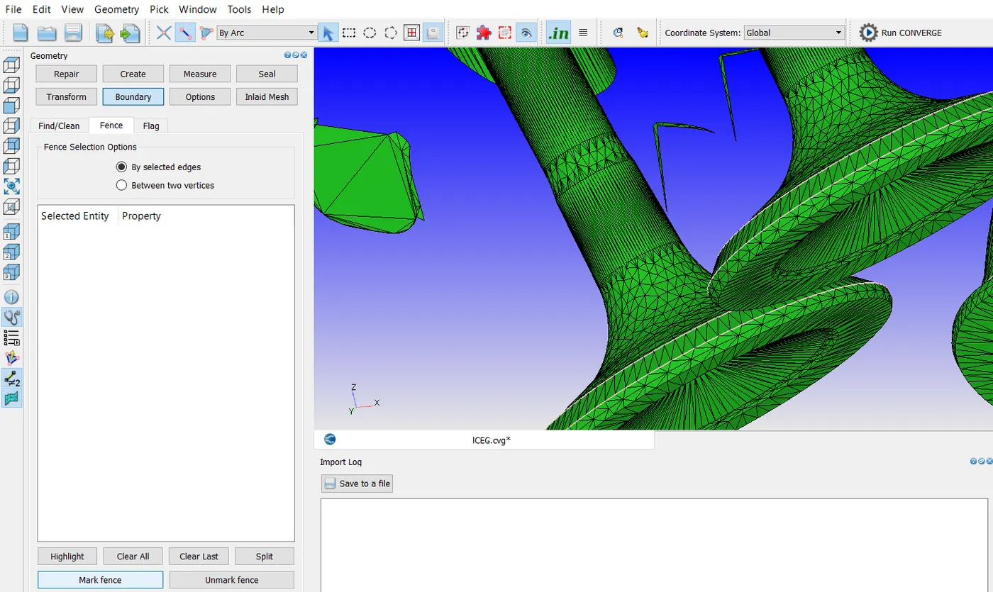
Now, the exhaust valve top boundary is flagged using the angle method as shown in the two images below.
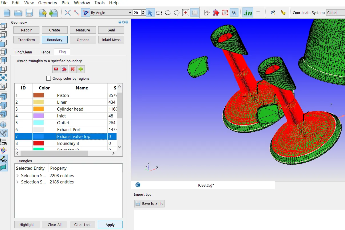
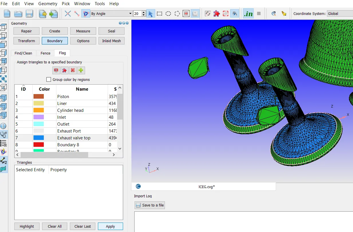
Now, the exhaust valve angle boundary is flagged using the boundary fence method as shown in the two images below.
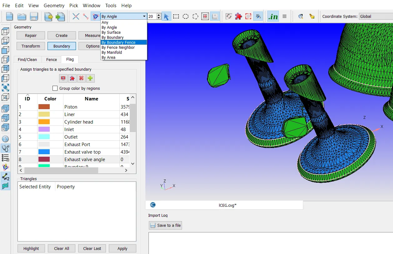
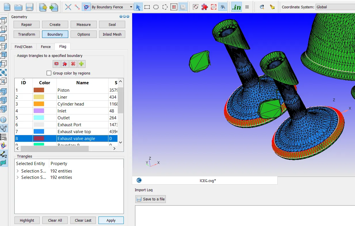
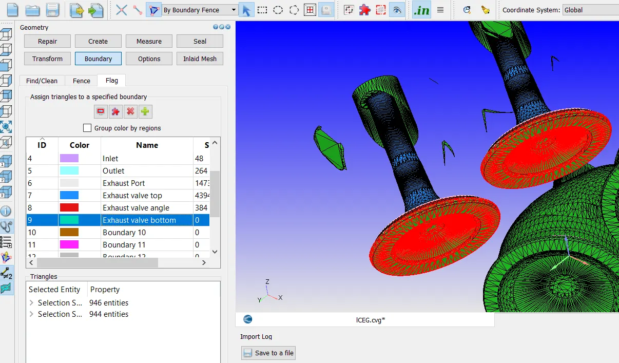
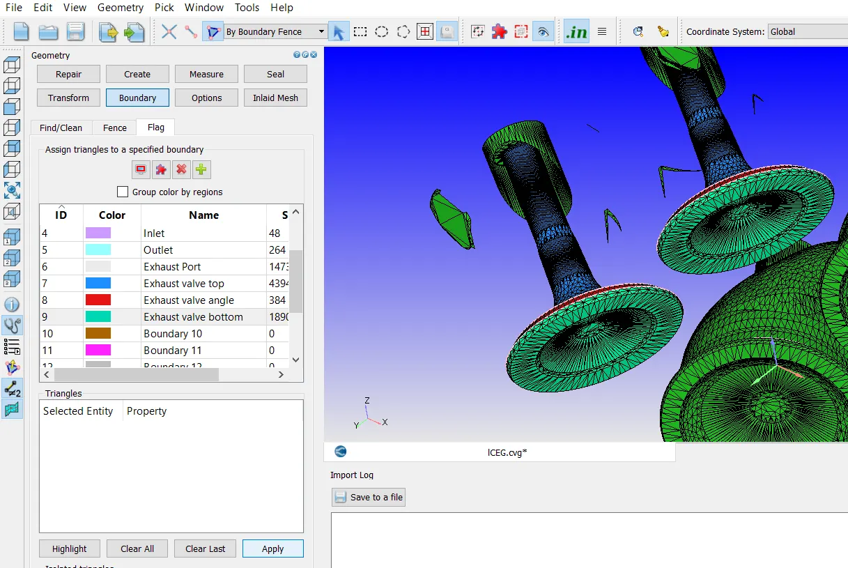
The exhaust valve bottom boundary is selected by using the boundary fence method and then flagged as shown in the below three images.
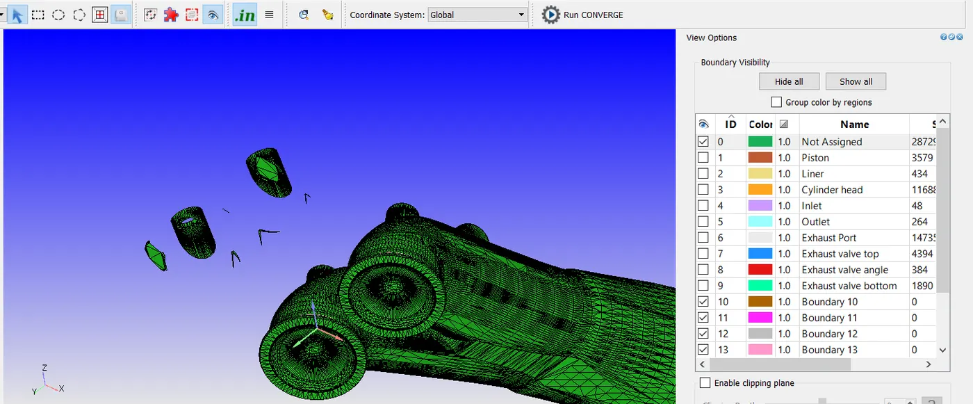
Now, the exhsust valve boundaries are hidden and the remaining portion of the exhaust port is selected as shown in the below two images.
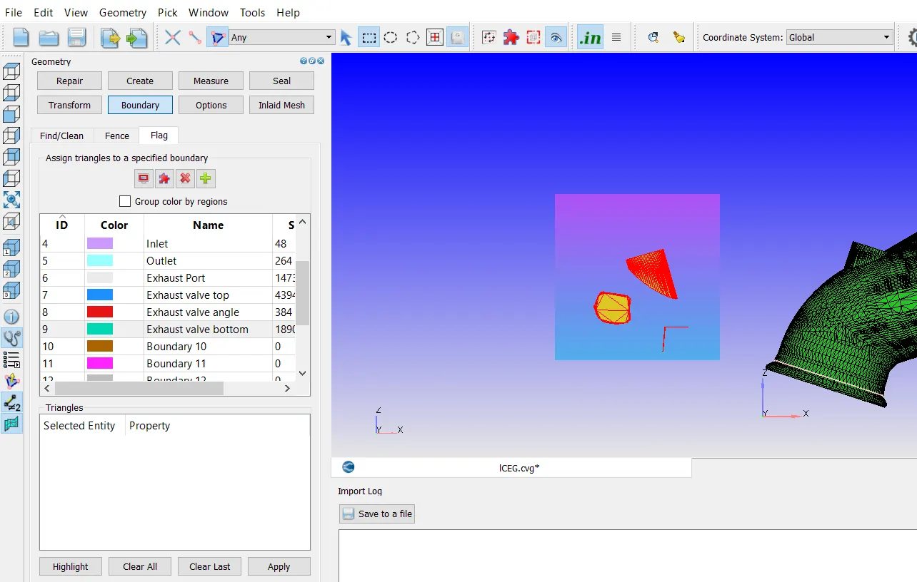
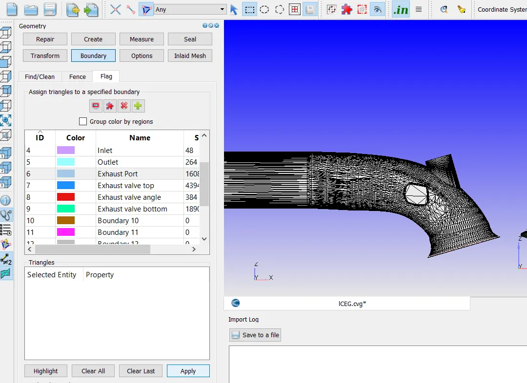
Now, the Exhaust port boundary is made visible and the selected portion is flagged to the exhaust port as shown in the image below.
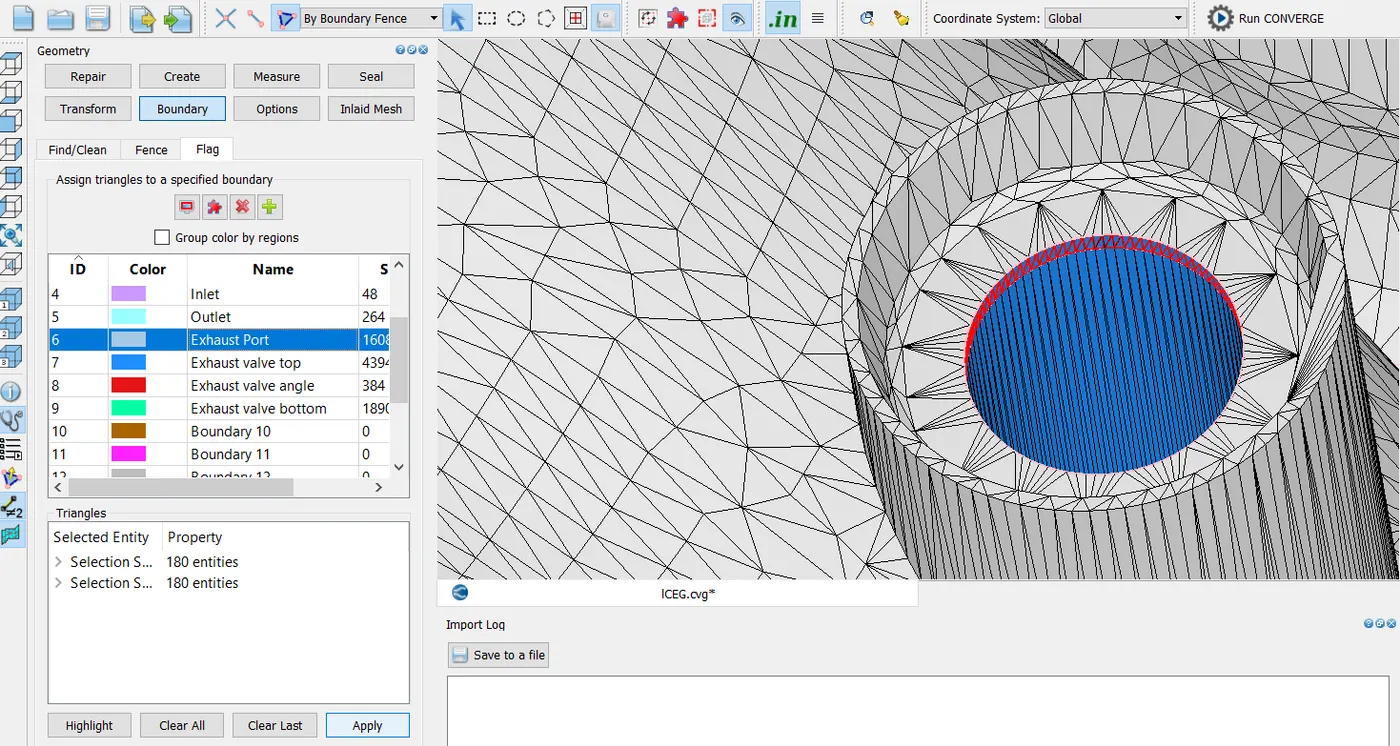
Now, boundary fences are marked for the rim triangles of the exhaust valve top as shown in the two images below.
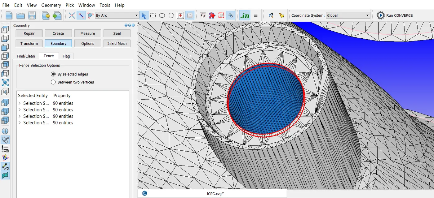
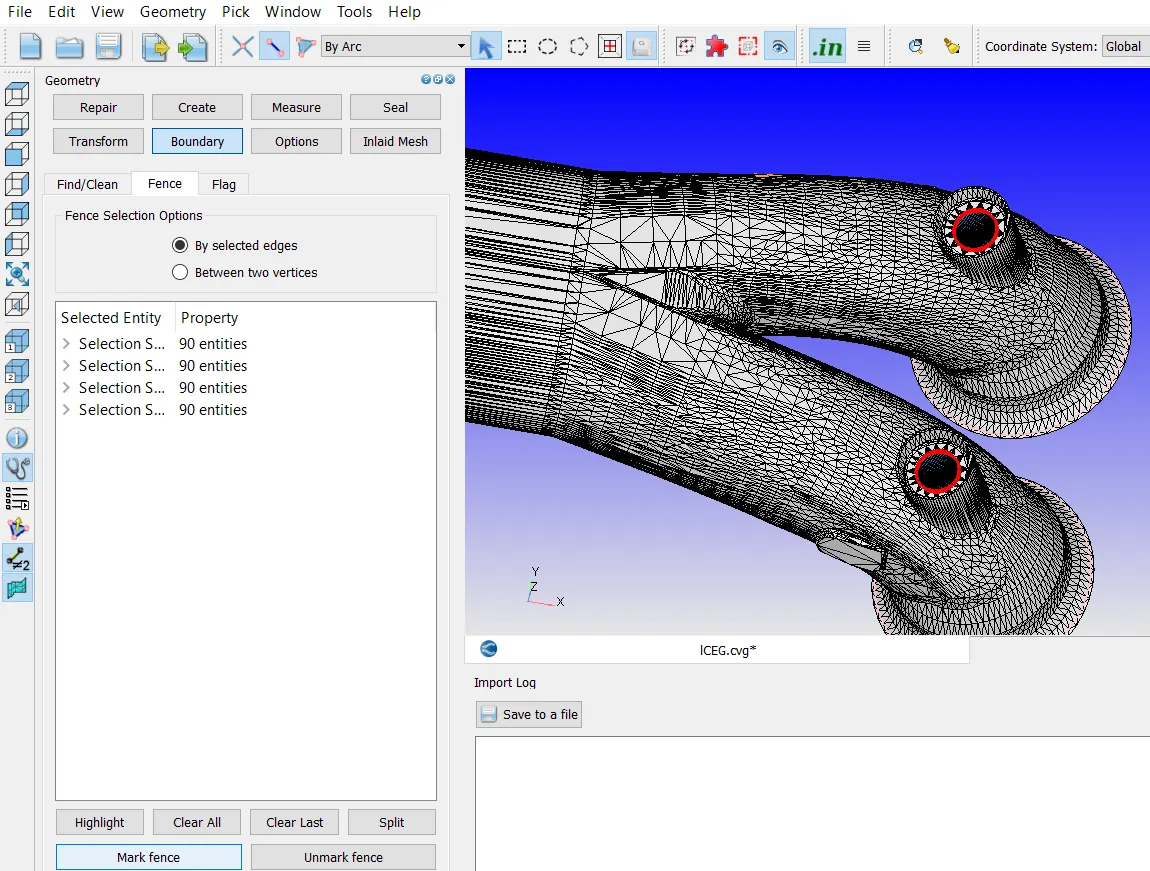
Now, these rim triangles are flagged to Exhaust port as shown in the below two images. This is done to avoid the distortion in shape of the portion of exhaust port near the rim triangles when it is required to translate the valve before setting up the case.
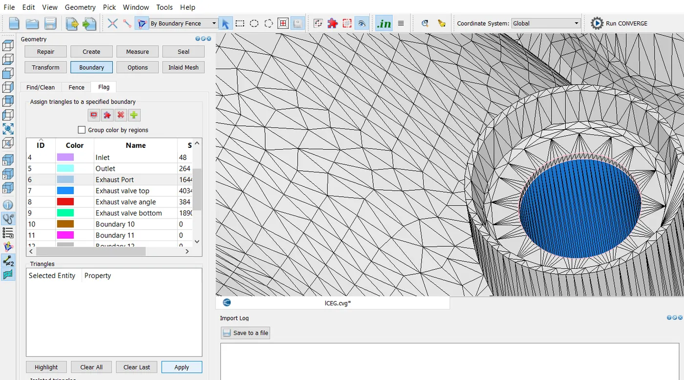
Now, all the bouondaries are redisplayed. Next boundaries which are going to be flagged are intake port and intake valves.
In the boundary fences, the option "reconstruct fences from existing boundaries" is clicked as shown in th eimage below.
Now, the boundary intake port is selected using the boundary fence method and flagged as shown in the below two images.
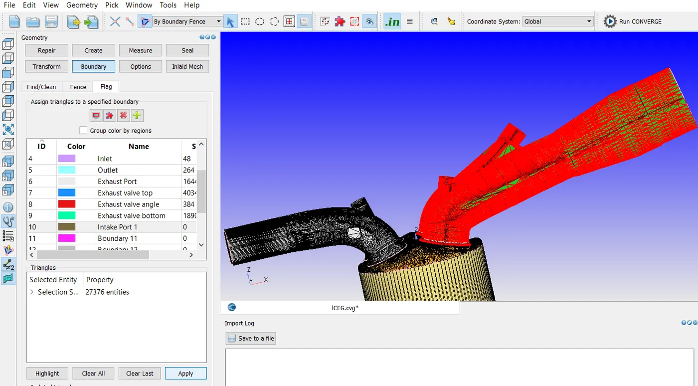
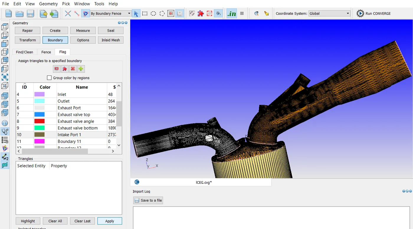
Now, all the boundaries are once again hidden except the intake port boundary so that the intake valves can be flagged.
Boundary fences are marked separating the intake valve top, angle, valve boundaries and the rim triangles at the intake valve top as shown in the below three images.
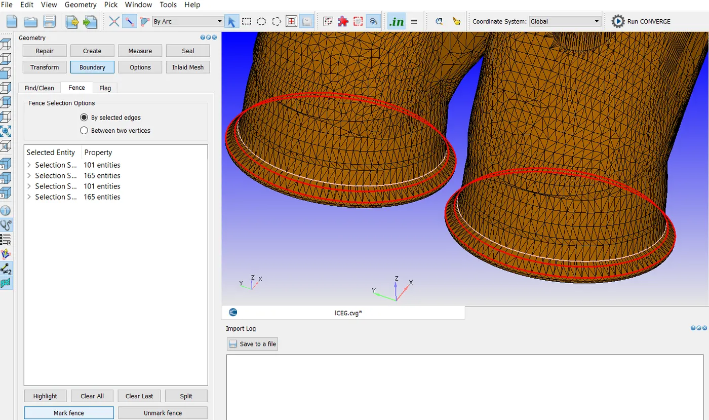
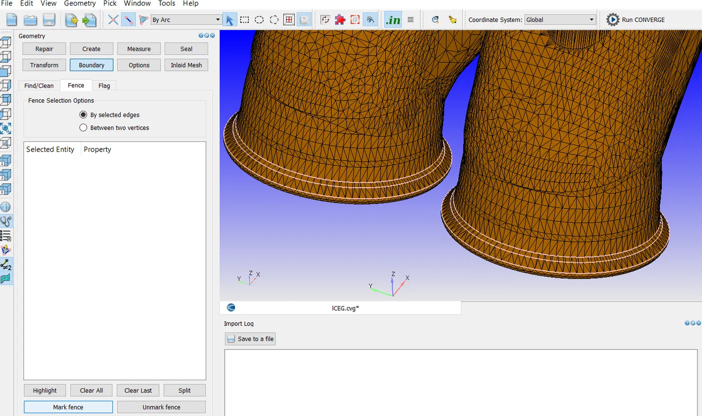
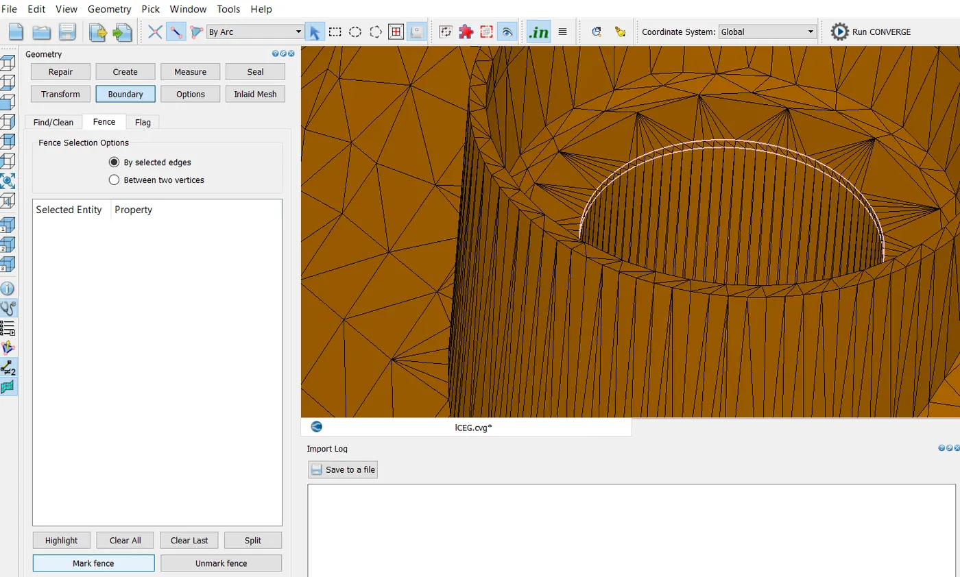
Now, the intake valve bottom is selected using the boundary fence method and then flagged as shown in the two images below.
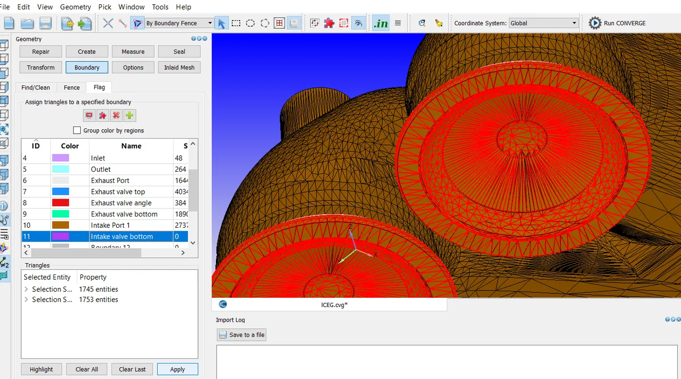
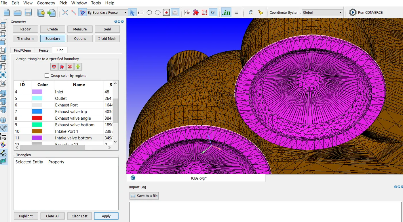
The intake valve angle is selected using boundary fence method and then flagged as shown in the below two images.
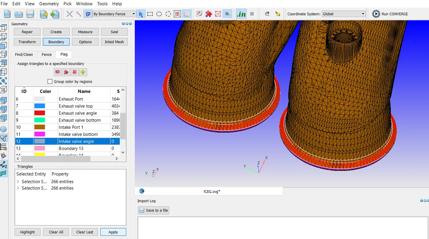
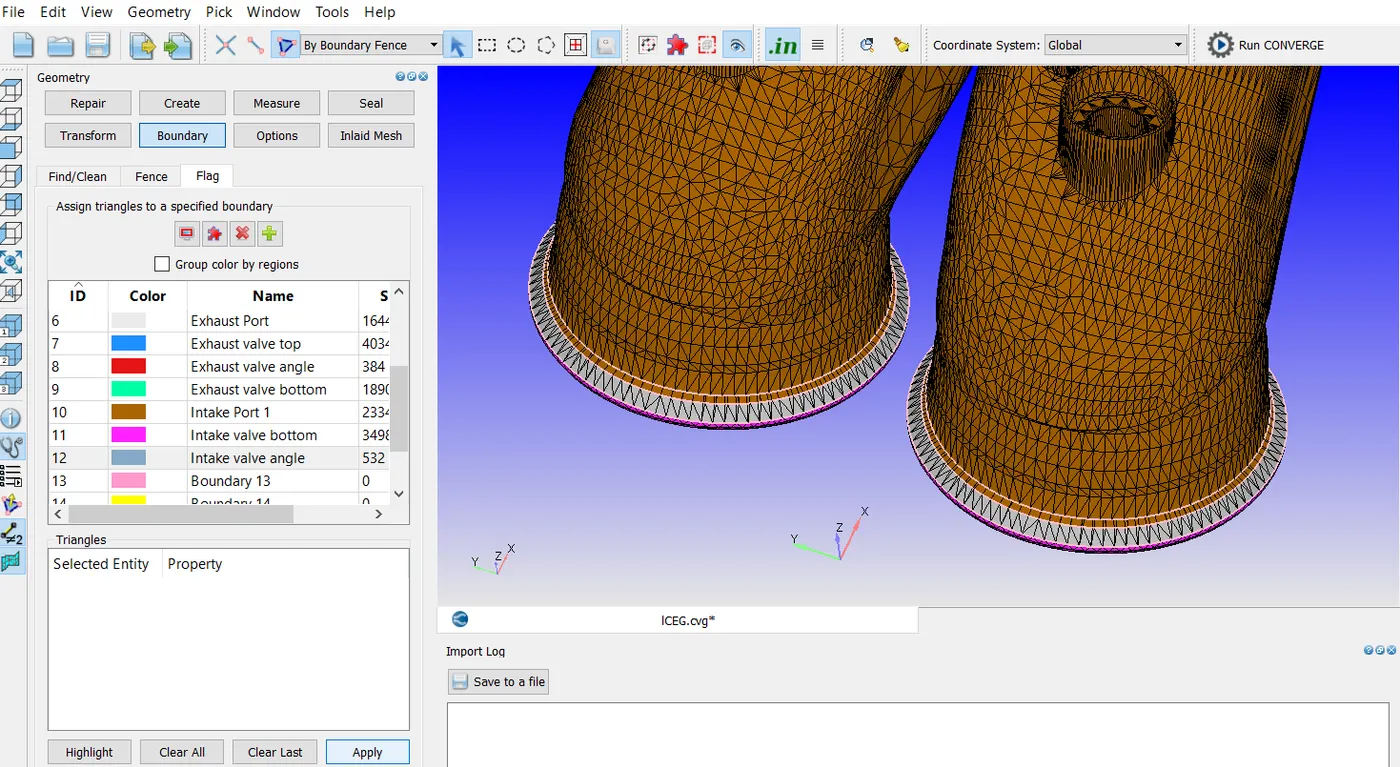
The intake valve top is selected using the boundary fence method and then flagged as shown in the below two images.
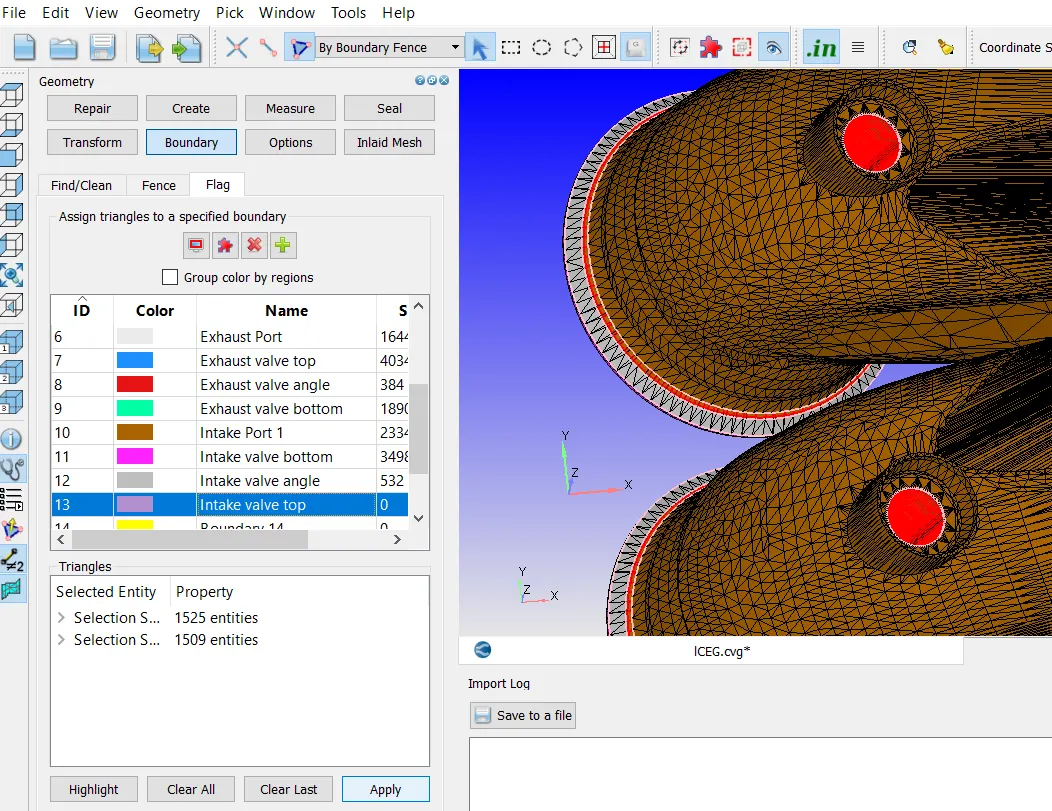
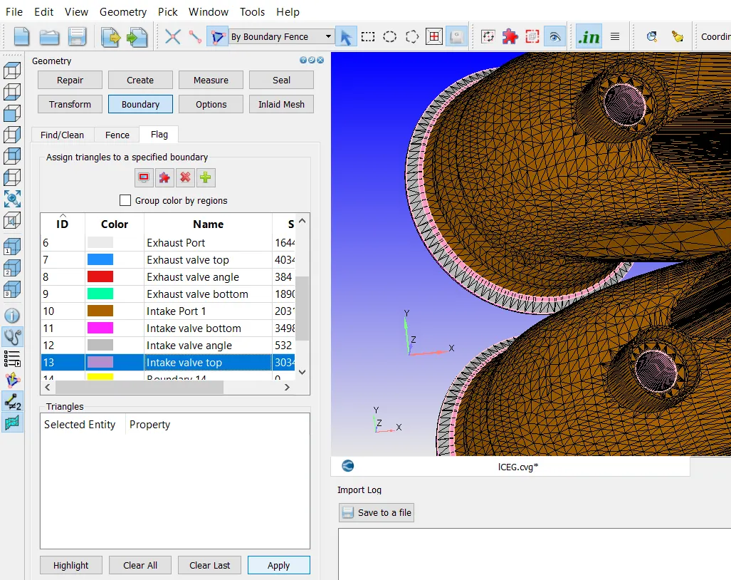
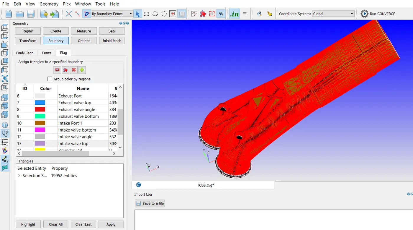
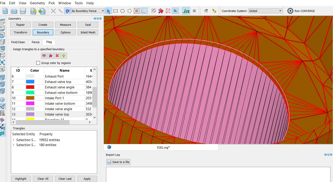
Now, the remaining portion of intake port along with the rim triangles is selected using the boundary fence method and then flagged as shown in the below three images.
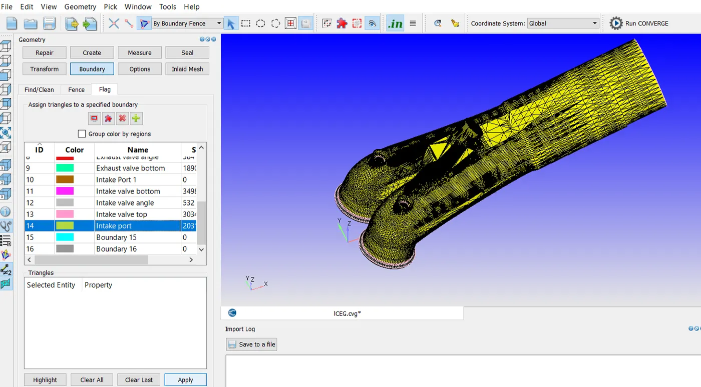
Now, all the boundaries are made visible except for piston, and liner as shown in the image below.
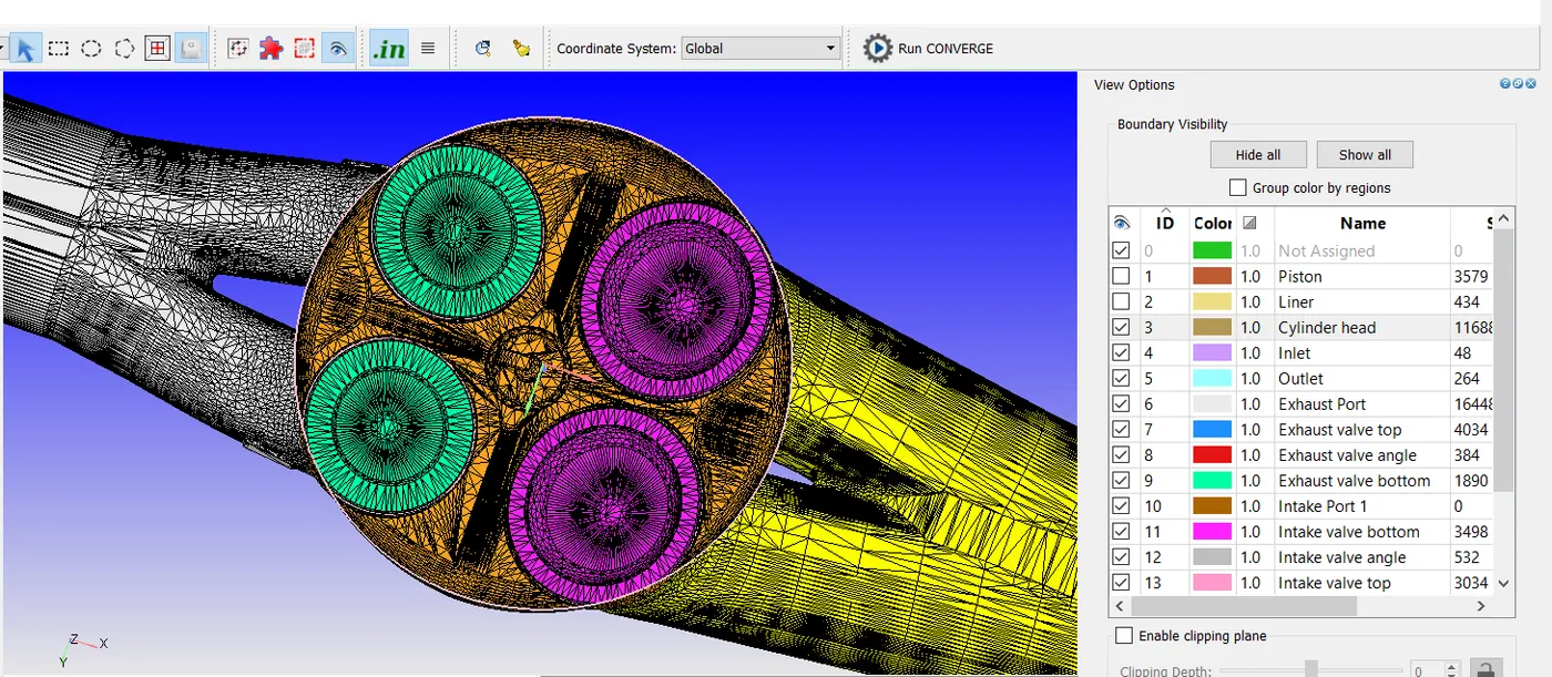
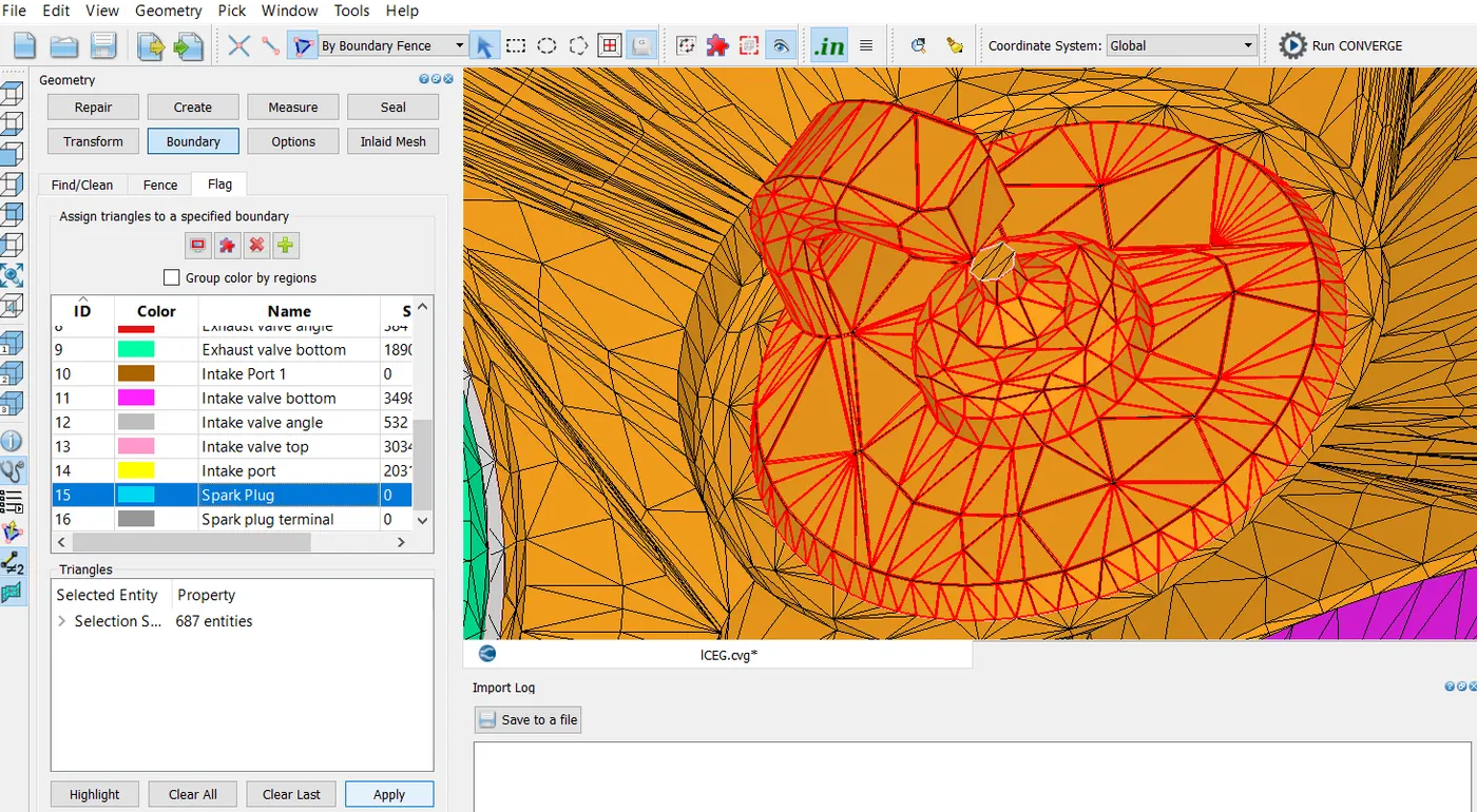
Now, the boundary fences are marked for separating the spark plug and the spark plug terminal as shown in the below two images.
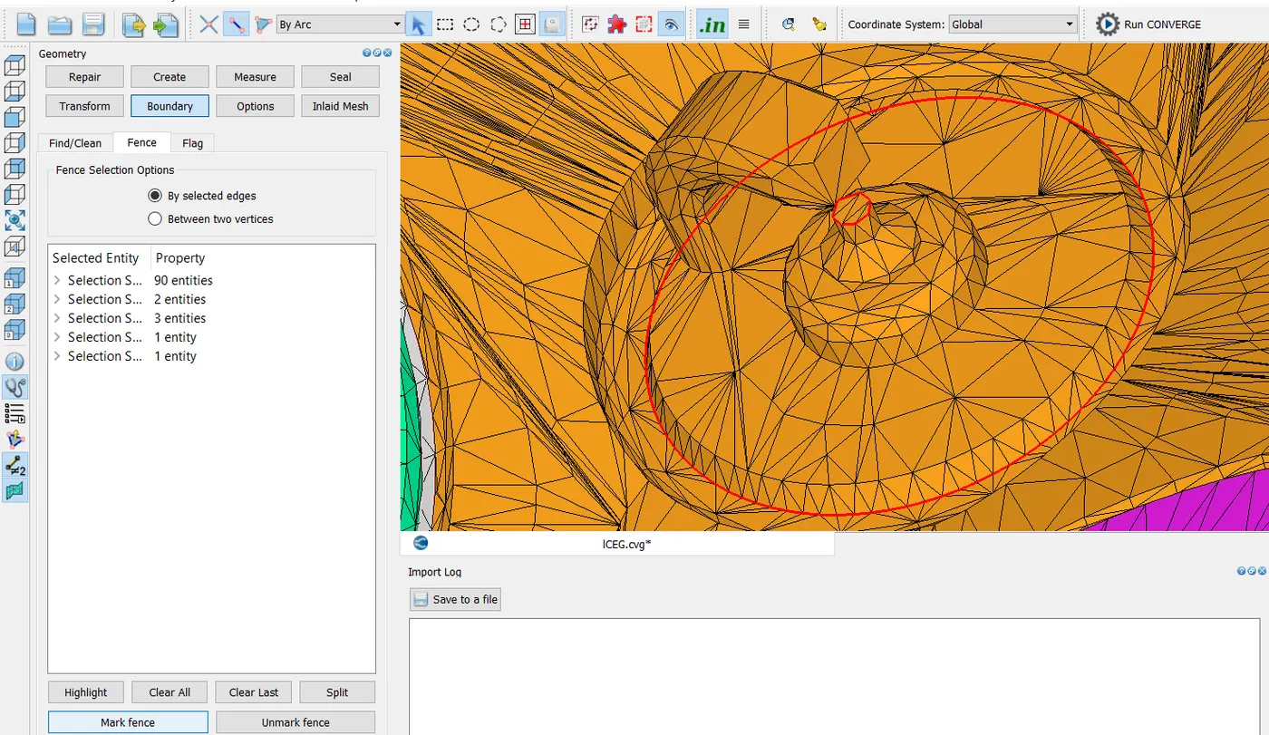
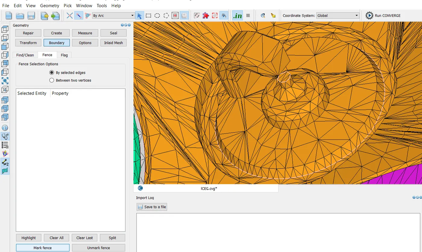
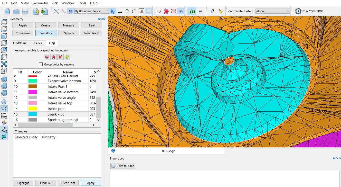
The spark plug boundary is selected using the boundary fence method and then flagged as shown in the below two images.
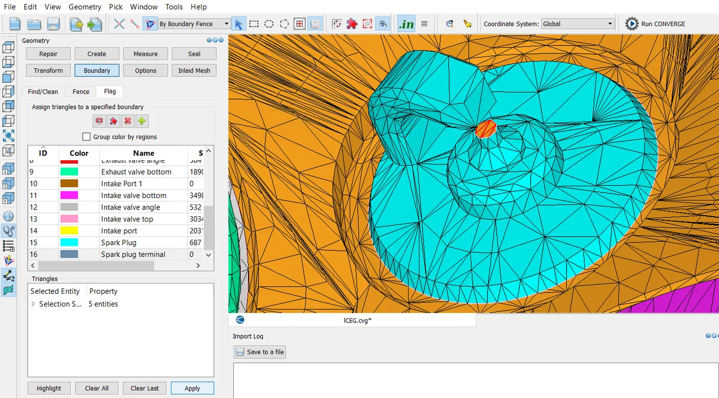
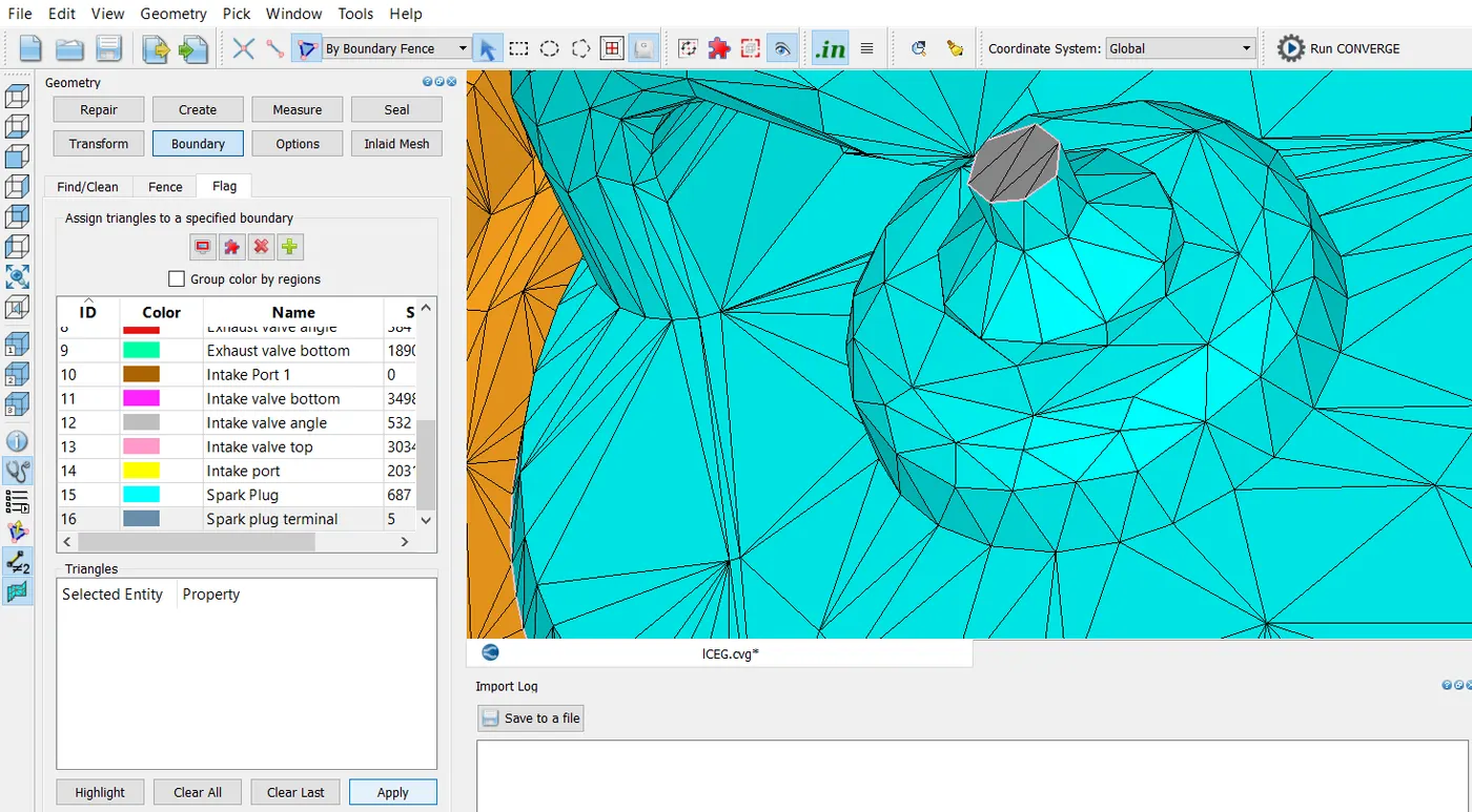
The spark plug terminal boundary is selected using the boundary fence method and then flagged as shown in the below two images.
Surface preparation:
Diagnosis:
Diagnosis of the geometry is done by clicking the find button in the dignosis dock as shown in the image below.
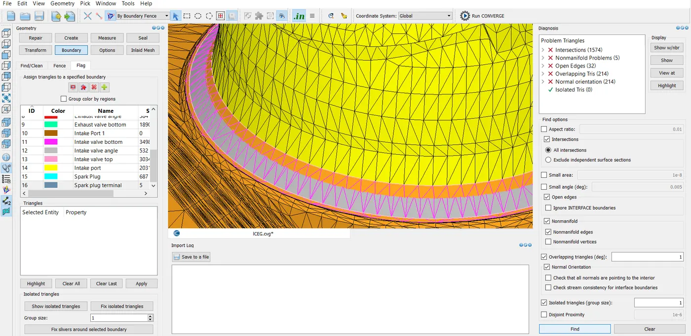
Also from the above image we can see that the cylinder head is intersecting with the intake valve boundary.
Now, to remove this error, the valve must be translated to some amount in the proper direction.
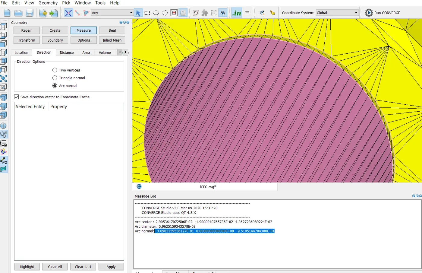
To do that the direction of the valve normal is measured under the measure section in the geometry dock. Three vertices method has been used to calculate the arc normal.
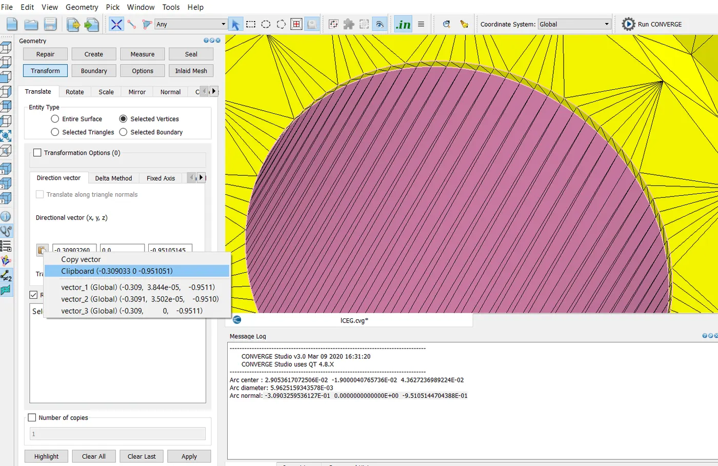
The arc normal is then copied and then pasted in the translate tab under transform section of the geometry dock and the entity type is seleced as selected boundary and then the three intake valve boundaries are selected and then small increaments of 0.0001m are made to correct the intersection. Corresponding images are shown below.
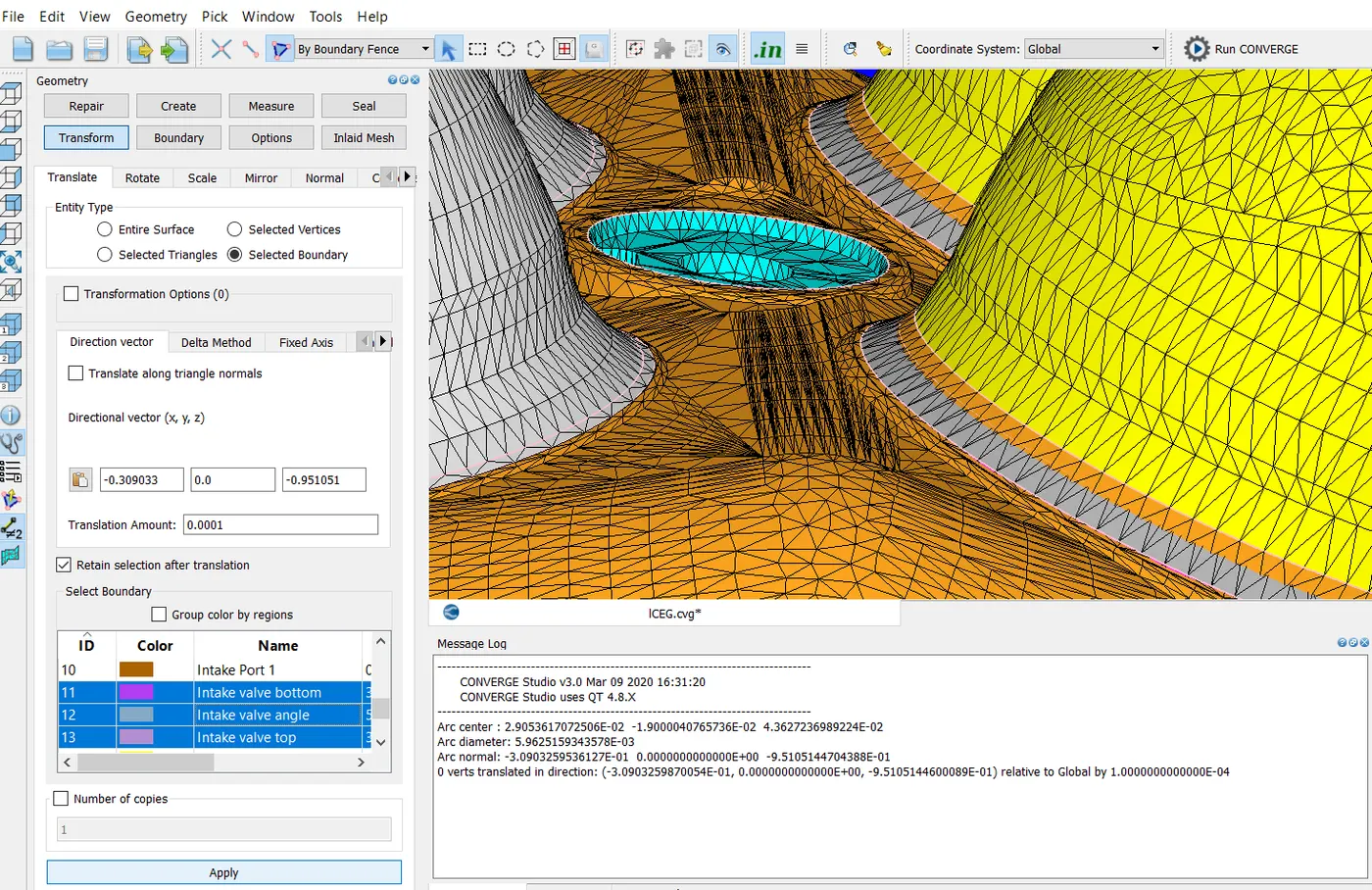
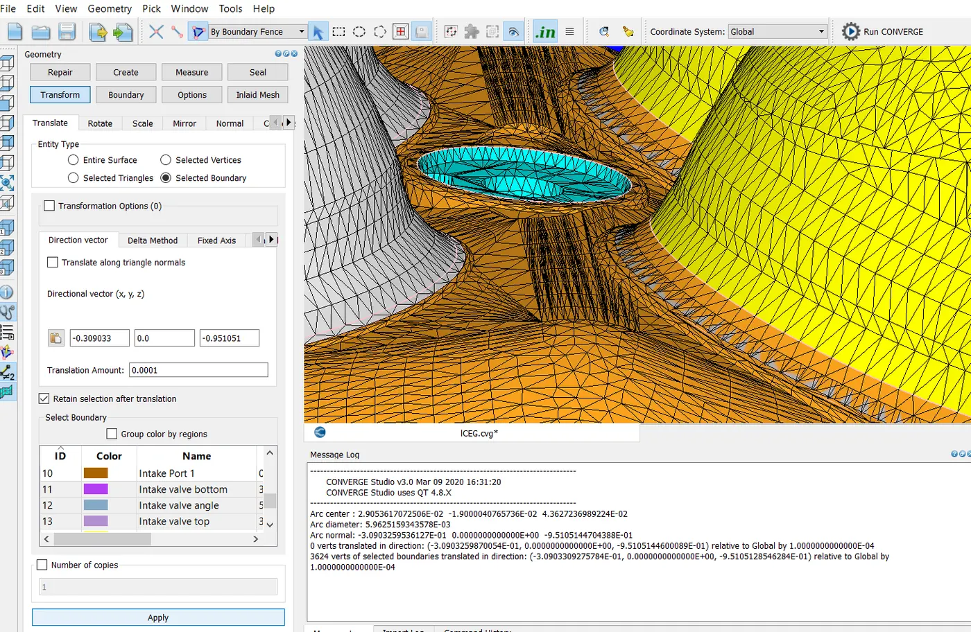
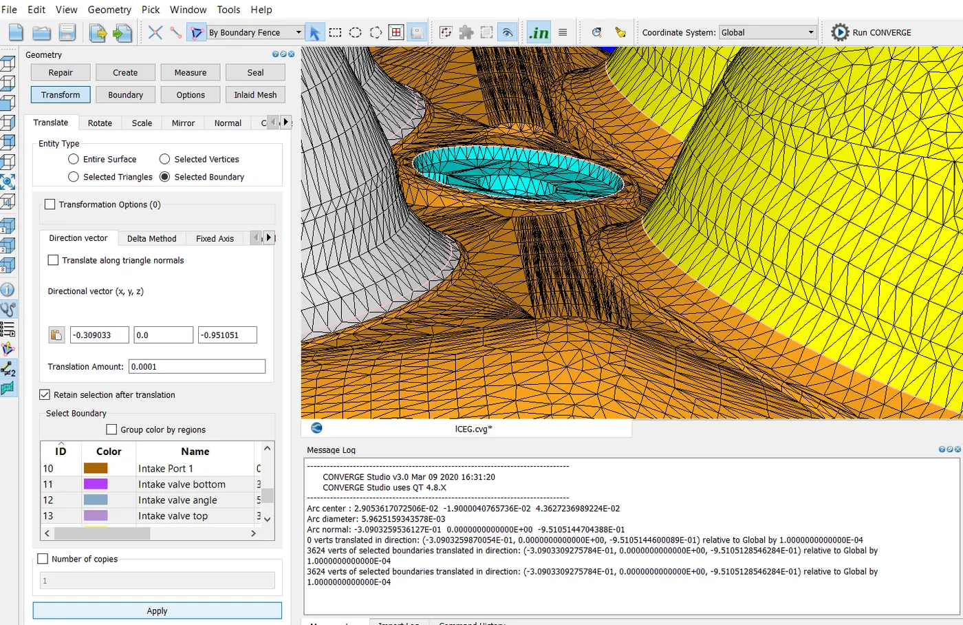
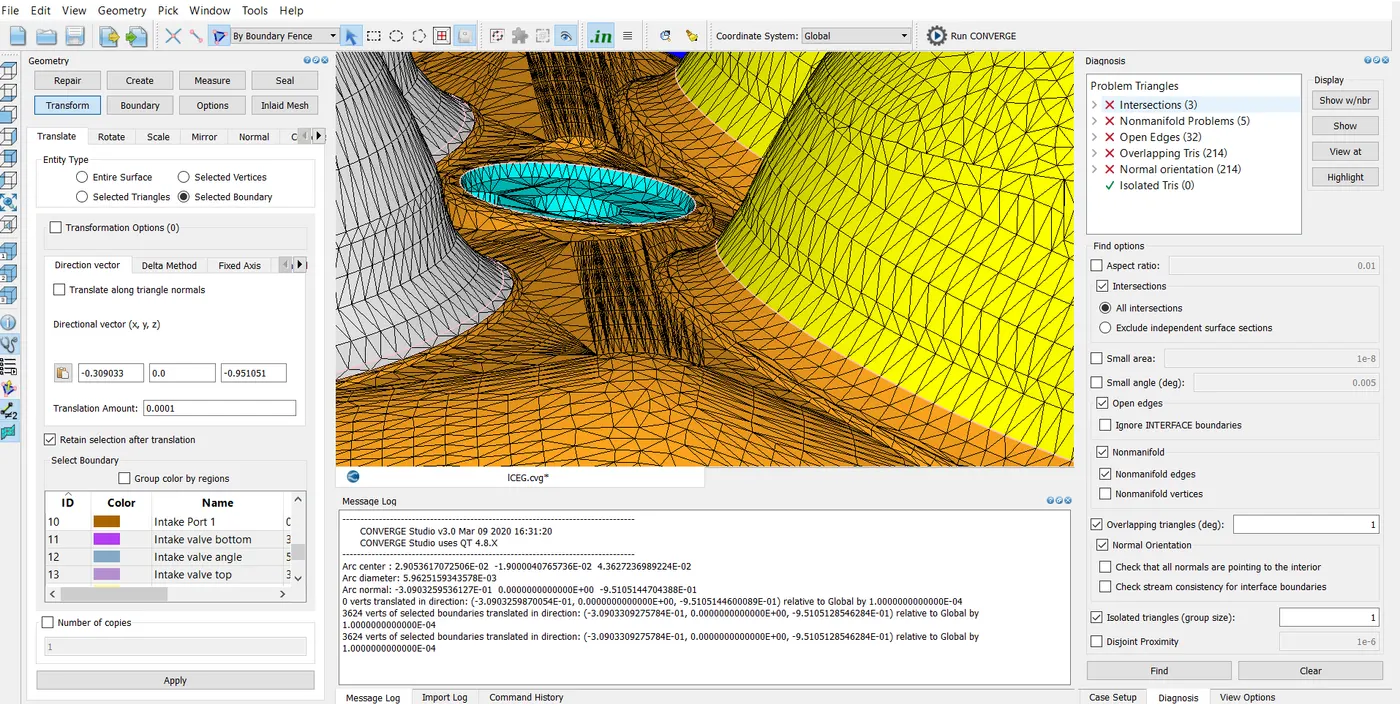
After diagnosing again the intersections are reduced to 3 as shown in the image below.
The piston has open edges as shown in the image below.
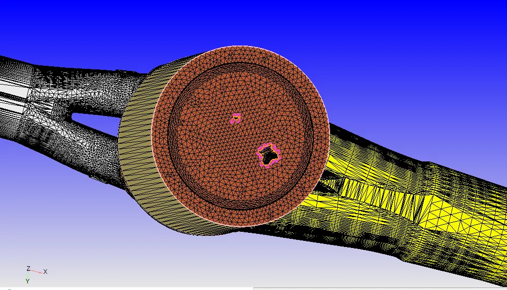
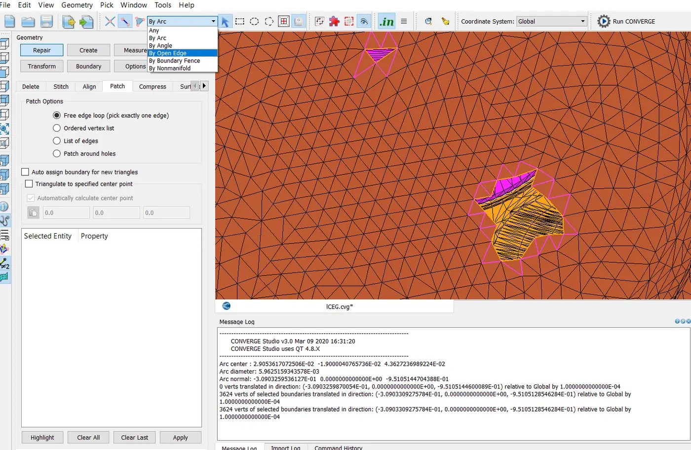
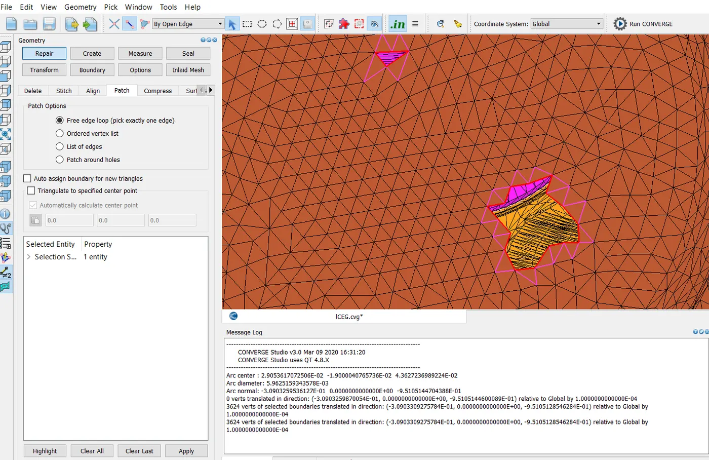
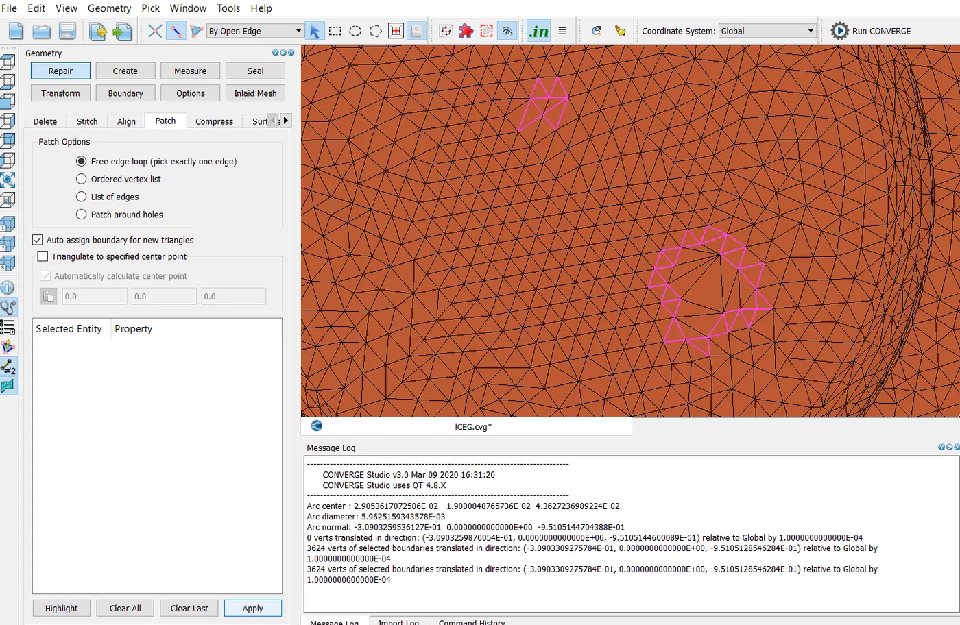
The open edges are fixed using the patch tool as the holes in the piston are not that big and they can retain the curvature.
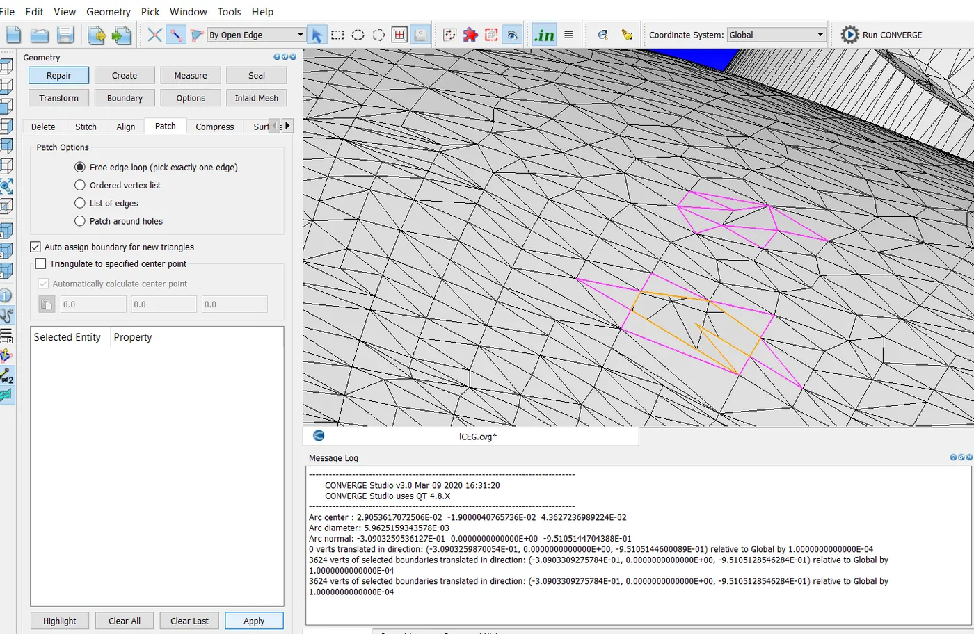
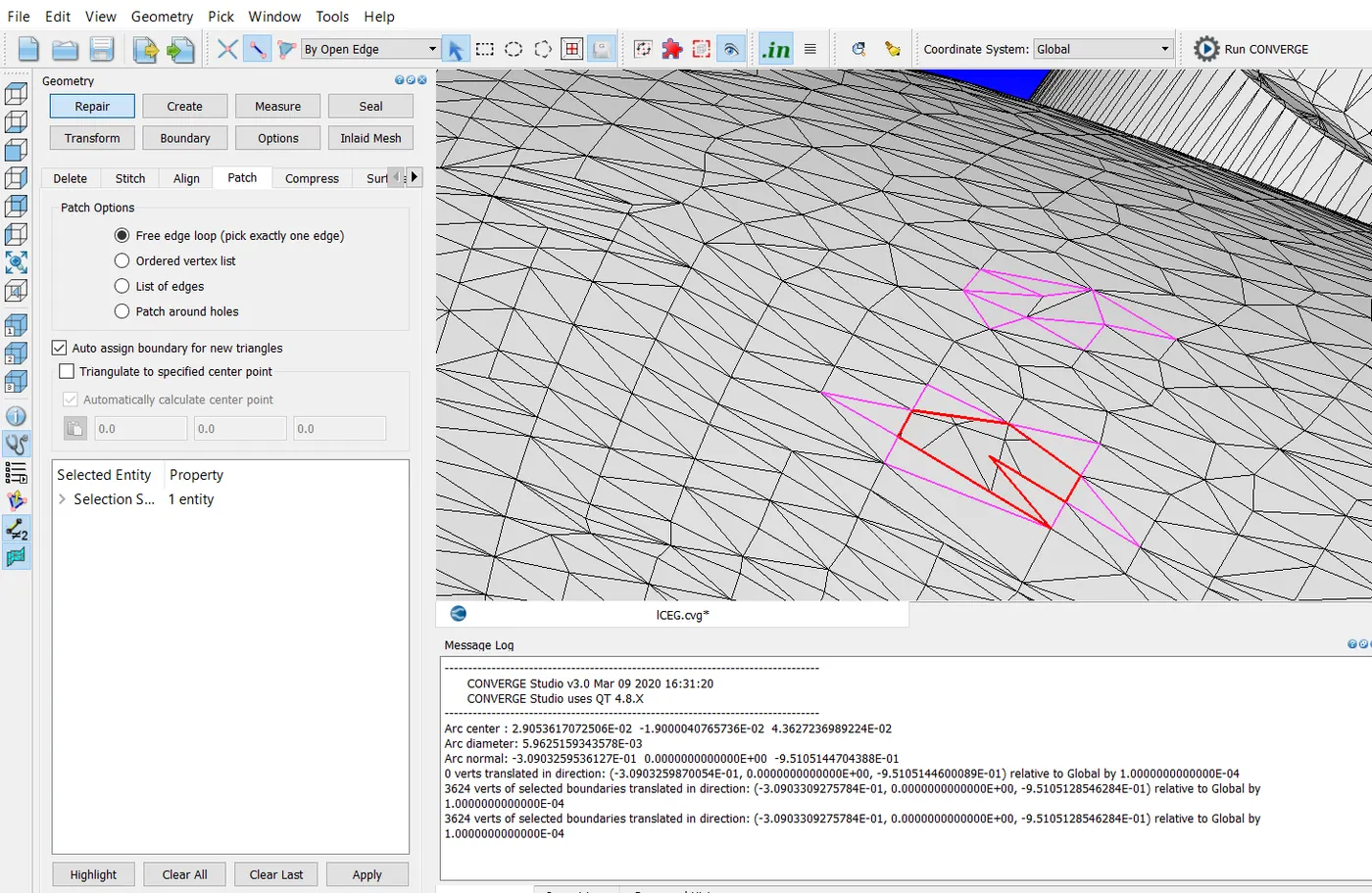
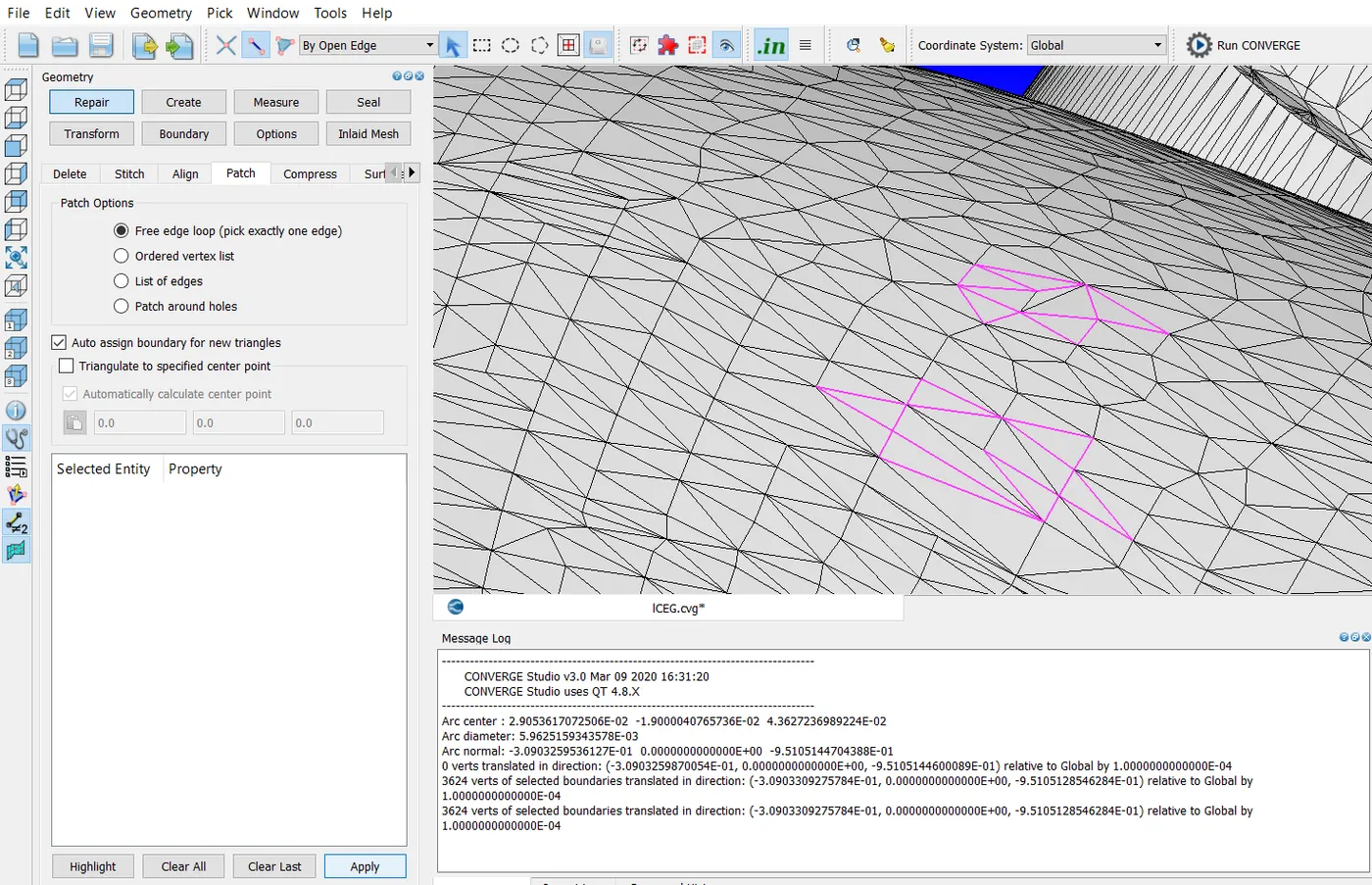
In the repair section of the geometry dock, select the patch tab and select the patch option free edge loop and then select the triangles by open edges and then check the box which says 'Auto assign boundry for new triangles'. After that patch the two holes in the piston. The corresponding images are shown below.
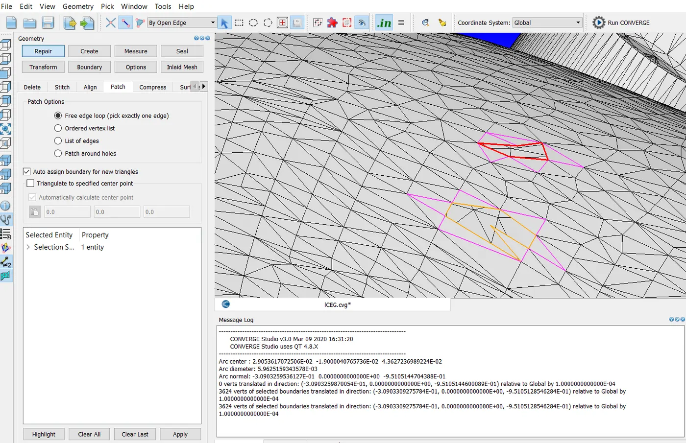
Similarly, the open edges on the exhaust port are closed by using the patch tool. The corresponding images are shown below.
Again diagnosis is run as shown in the image below.
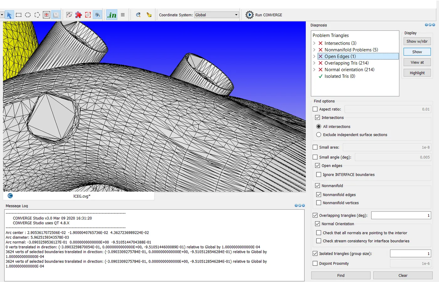
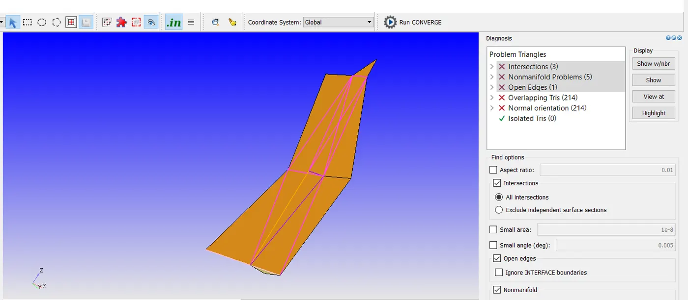
It can be observed from the above image that the open edges have been reduced to 1.
Now, we select the intersection, non-manifold problems and open edges and click the show option to see these errors as shown in the image below.
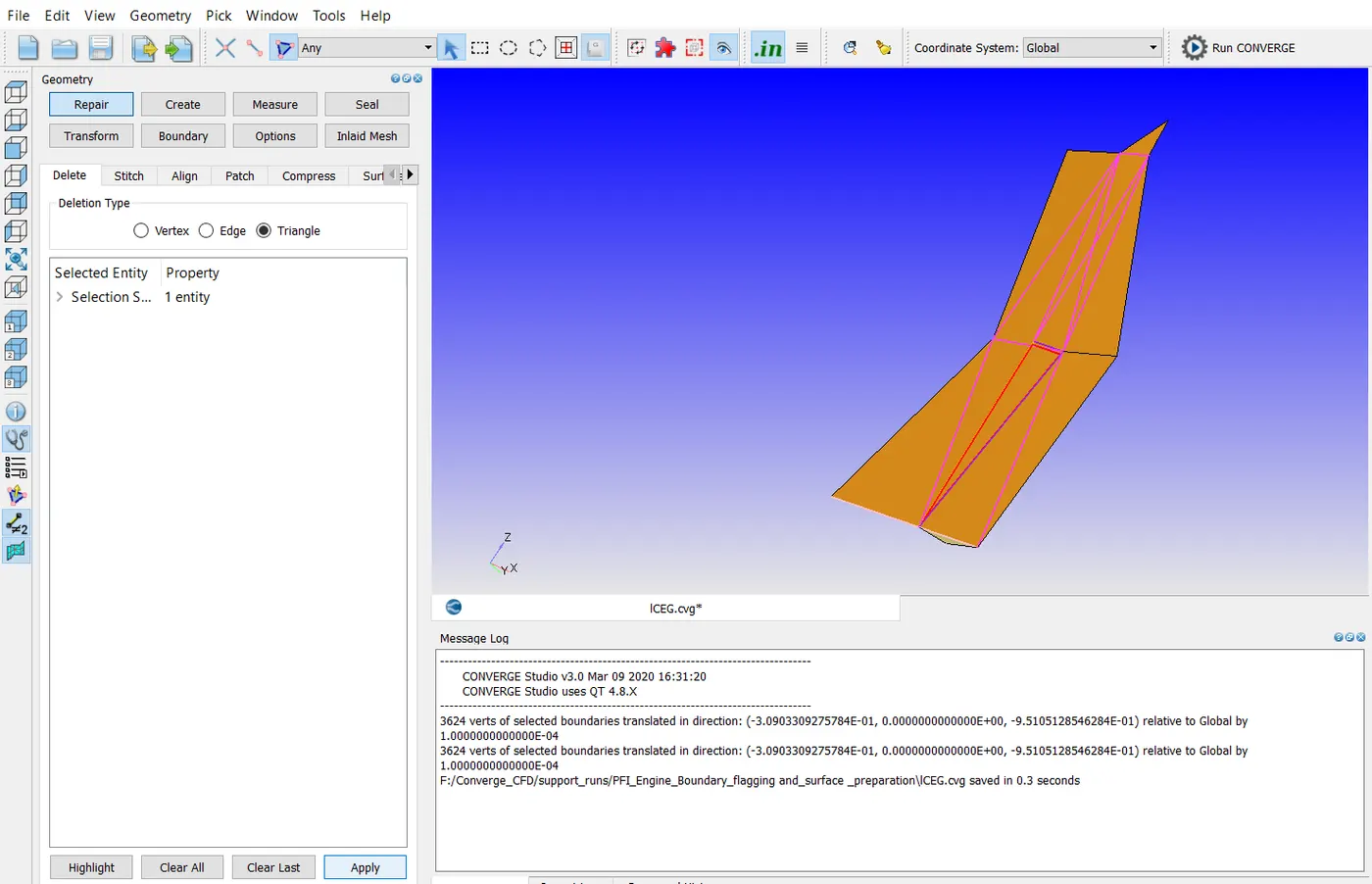
The open edge is selected as shown in the below image.
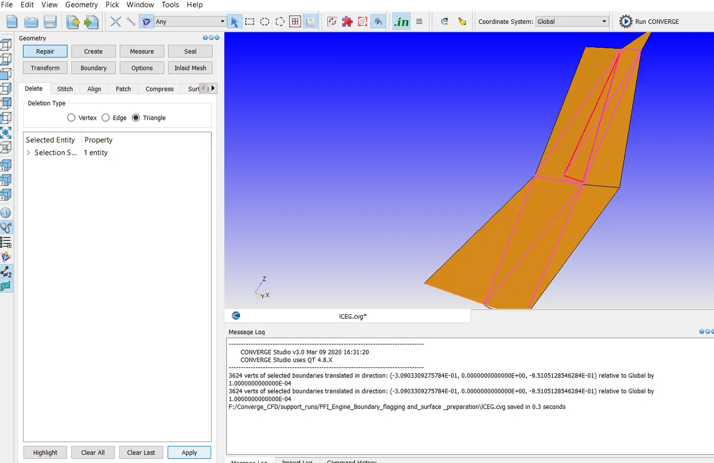
The open edge is deleted and the intersecting triangle is selected as shown in the image below.
The selected intersecting triangle is deleted and another intersecting triangle is selected as shown in the image below.
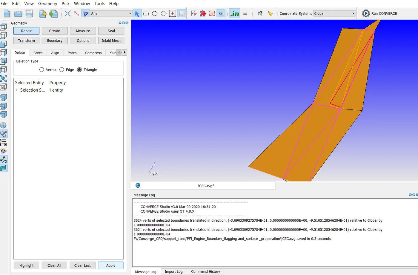
The selected intersecting triangle is deleted and a non-manifold problem triangle is selected as shown in the image below.
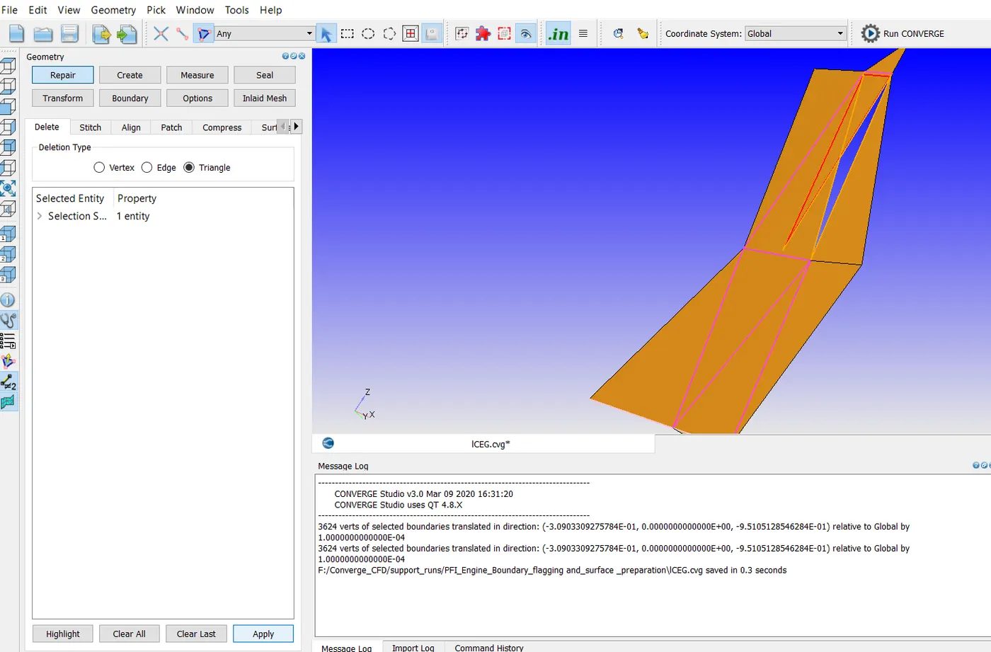
The non-manifold problem triangle is deleted and then the open edge loop is selected to patch as shown in the image below.
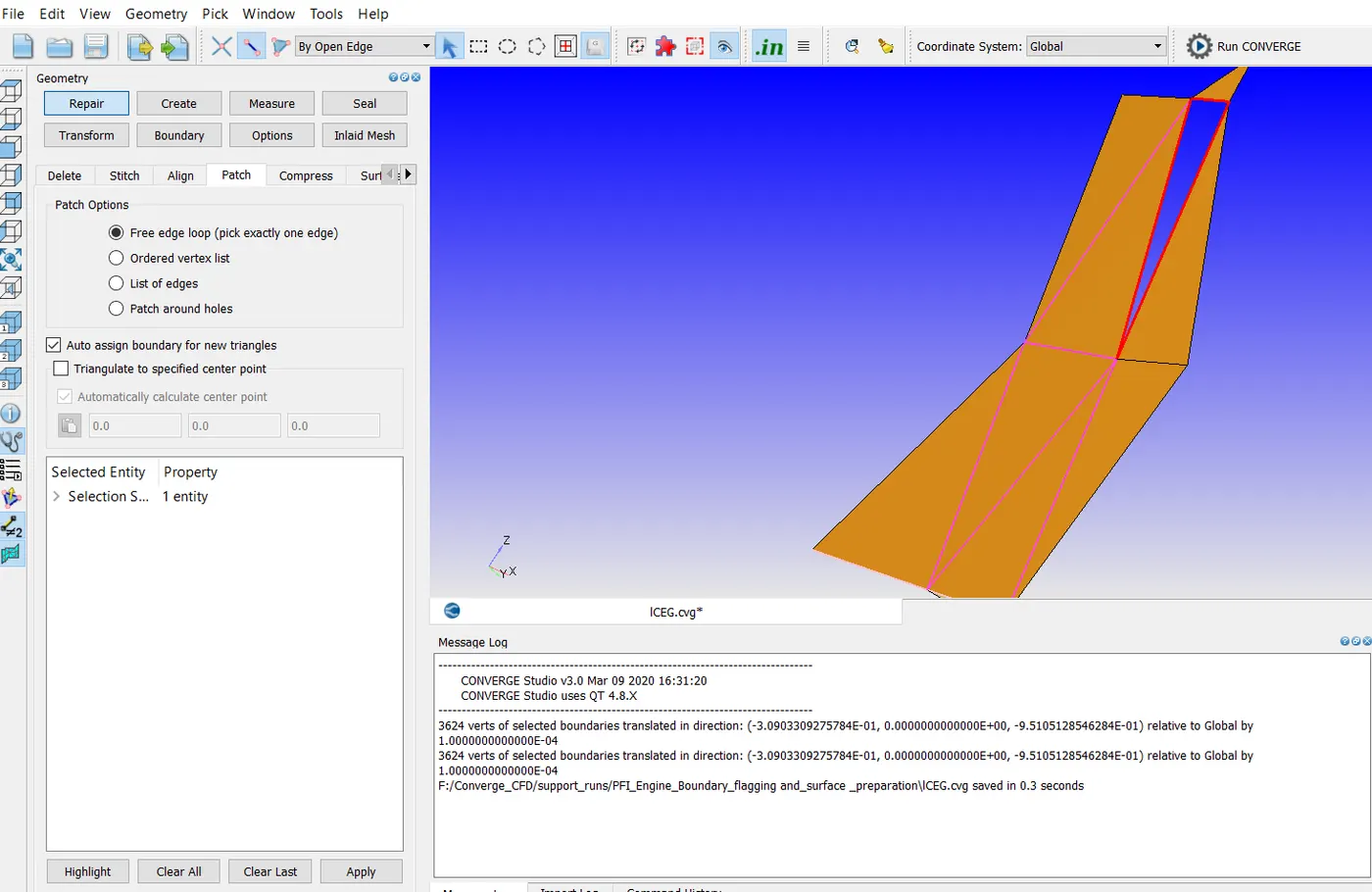
The open edge loop is closed using the patch tool as shown in the image below.
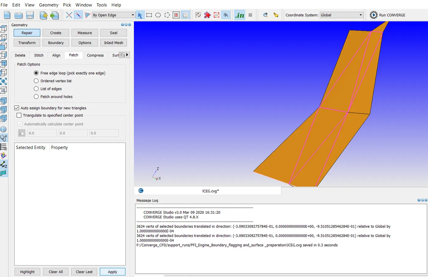
Diagnosis is performed once again and the next problem to be fixed is normal orientations.
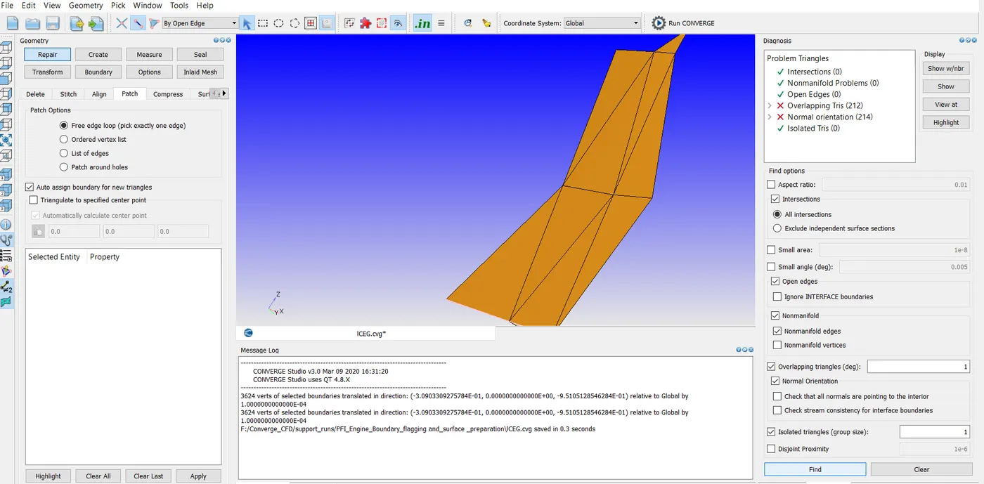
In the transform section of geometry dock, Normal tab is seected and the normal icon is clicked which is present in the extreme left column in the image below which is third from the bottom to see the normals. Then, one of the triangles is selected as shown in the image below.
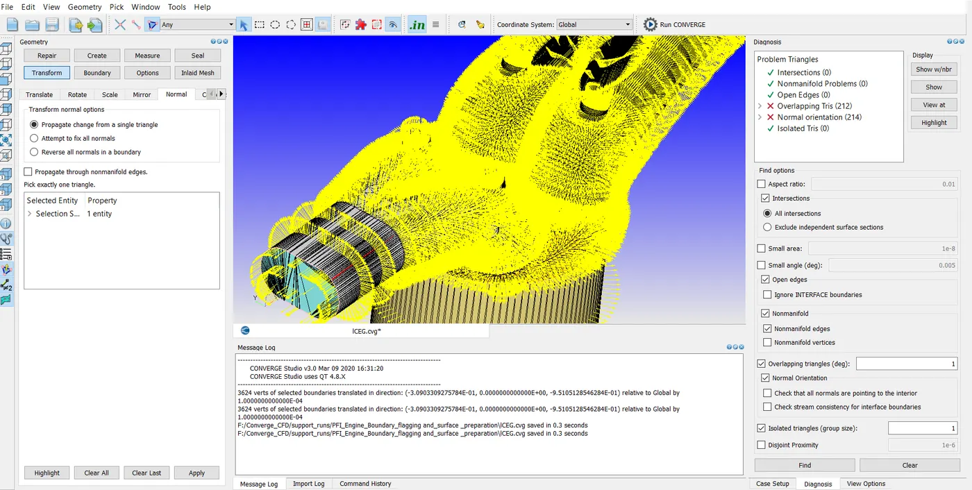
Apply option is clicked and the normals are pointing inside the PFI engine. The normal orientations problem has been solved and the diagnosis is done once again and it has been found that there are no problem triangles as shown in the image below.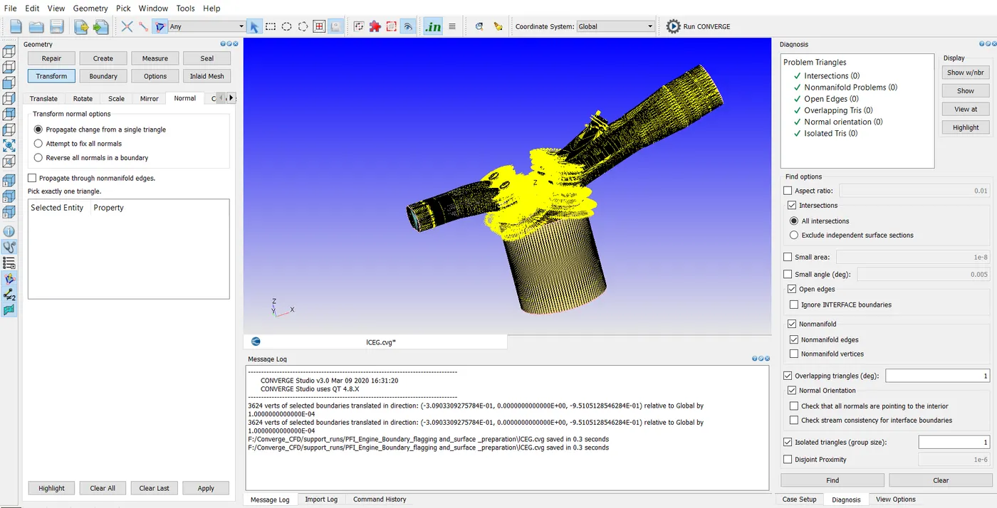
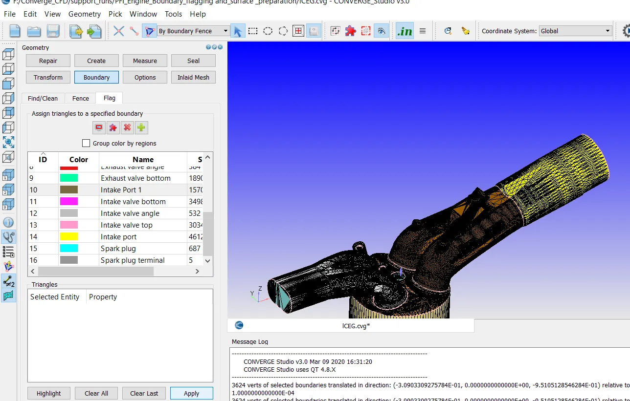
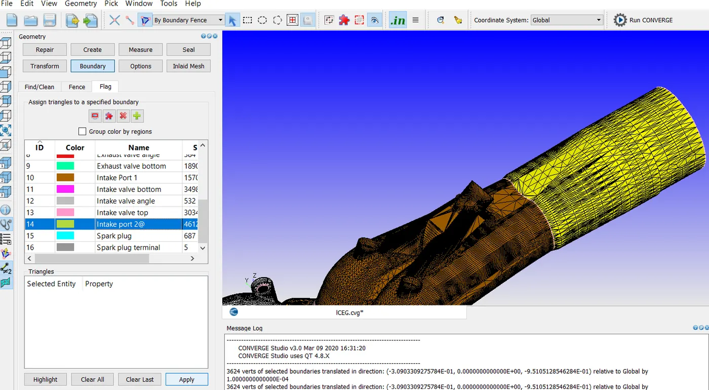
Now, the intake port is divided into two parts intake port 1 and intake port 2, so that we can provide initial condition seperately for intake port 1 and intake port 2 as the fuel is injected in the intake port 1.
A boundary fenc eis marked to separate intake port 1 aand intake port 2 using the arc method under selected edges method as shown in the below two images.
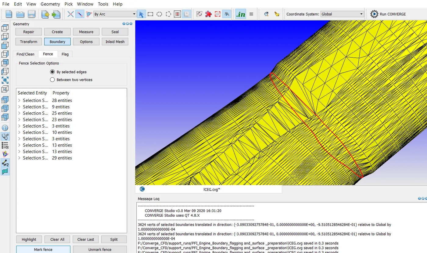
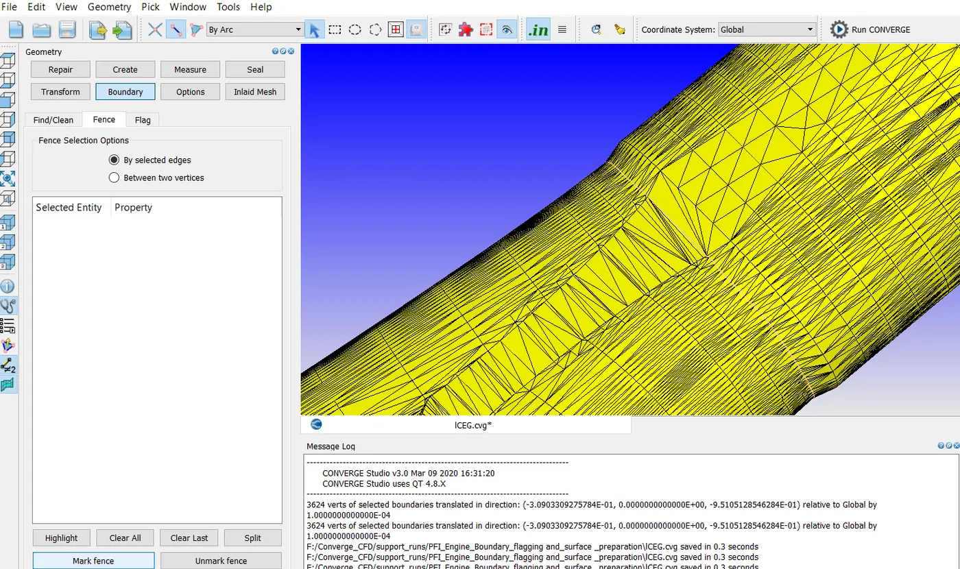
By using the boundary fence method, the inlet port 1 and inlet port 2 are selected and flagged as shown in the below two images.
CASE SETUP:
As the geometry now has cleared the diagnosis, setting up the case is the next step. Here, no hydro simulation case setup is done. This means that there are no equations sto be solved. This setup checks the generation of mesh and the feasibility to run the simulation.
Following files are used as an input:
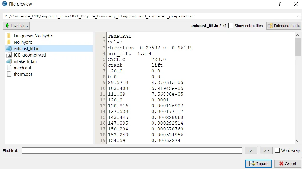
This file contains the exhaust valve profile at different crank angles during the simulation.
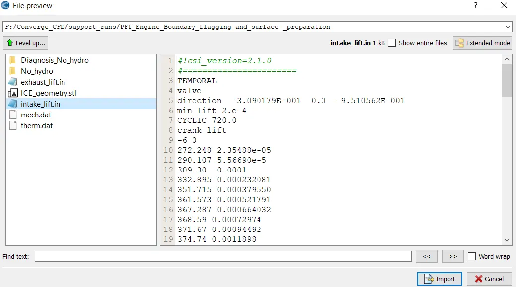
This file contains the exhaust valve profile at different crank angles during the simulation.
c) mech.dat
This file contains the PRF reaction mechanism which is involved in the combustion of fuel.
d) therm.dat
This file contains the thermodynamic properties of the chemicals involved in the combustion.
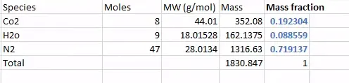
The combustion reaction is assumed to be stoichiometric and the balanced reaction is shown below.
`C_8H_18 + 12.5.(O_2 + 3.76N_2) -> 8CO_2 + 9H_2O + 12.5*3.76N_2`
The mass fraction calculations are shown below:
1) Application type:
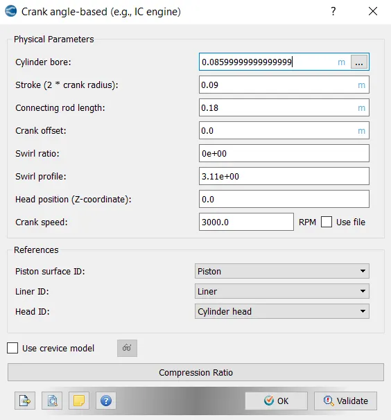
The appliction type is seected as 'Crank angle-based IC Engine'
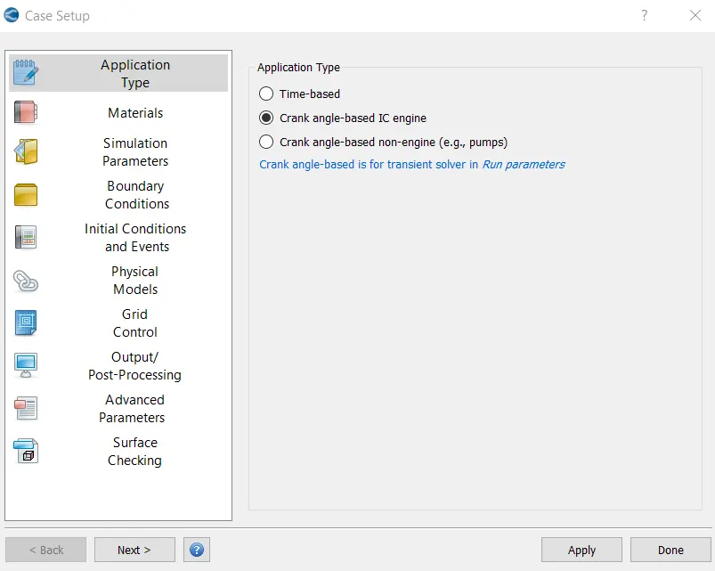
Under the Crank angle-based IC Engine, the following are set.
Cylinder bore: 0.086 m
Stroke: 0.09 m
Connecting rod length: 0.18 m
Crank offset: 0.0 m
References are set as:
Piston surface ID: Piston
Liner ID: Liner
Head ID: Cylinder head
2) Materials:
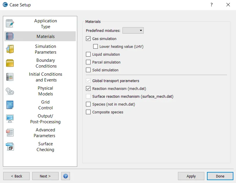
In the materials section, Gas simulation and Reaction mechanism are checked.
i) Gas simulation:
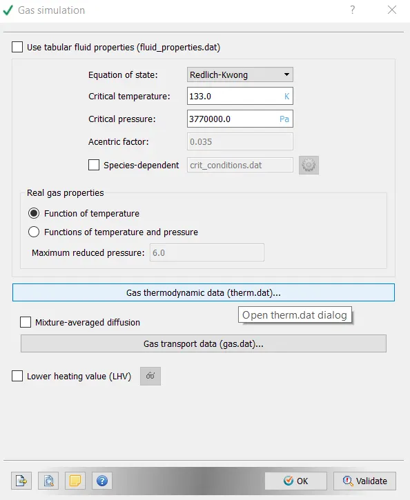
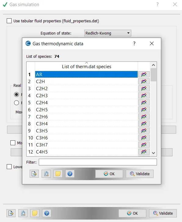
In gas simulation the gas thermodynamic data(therm.dat) is clicked and it is validated as shown in the below two images.
ii) Global transport parameters:
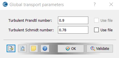
Global transport parameters are set as default as shown in the image below.
iii) Reaction mechanism:
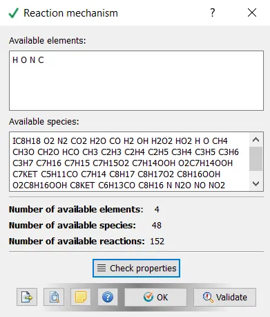
In the reaction mechanism, check properties is clicked and then it is validated.
3) Simulation parameters:
i) Run parameters:
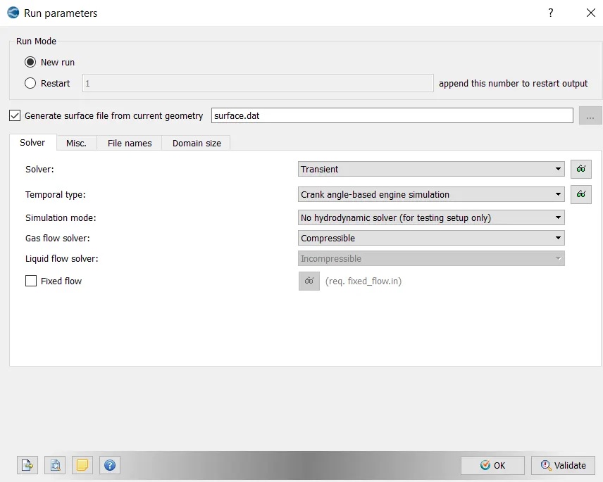
In run parameters, the solver type is selected as Transient and the simulation mode is selected as No hydrodynamic solver.
ii) Simulation time parameters:
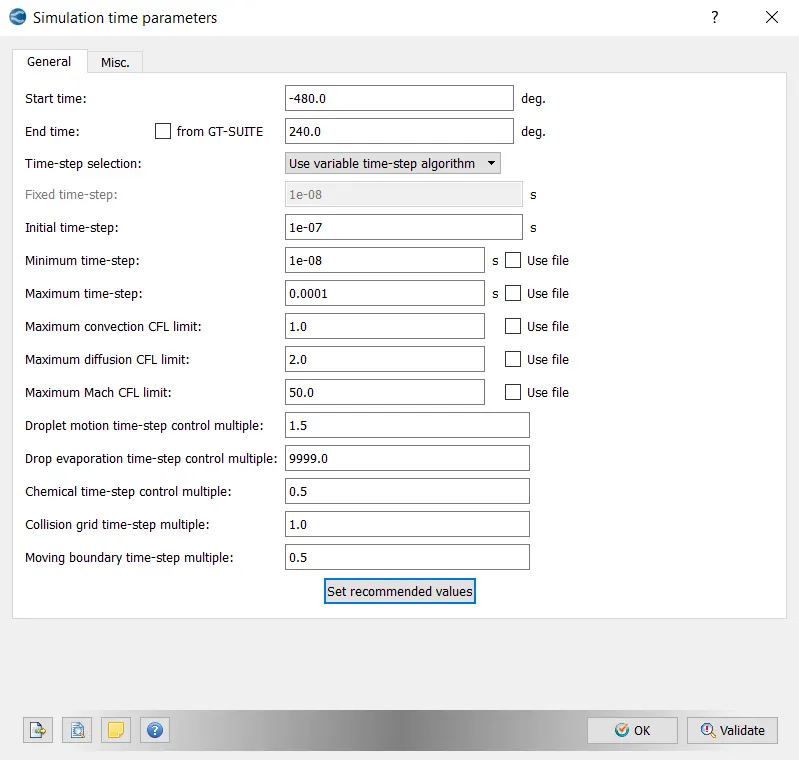
Under the simulation time parameters the conditions are set as following:
1) start time = -480.0 degrees
2) End time = 240.0 degrees
3) Initial time step = 1e-7 s
4) Minimum time step = 1e-8 s
5) Maximum time step = 0.0001 s
6) Maximum convetion cfl limit = 1.0
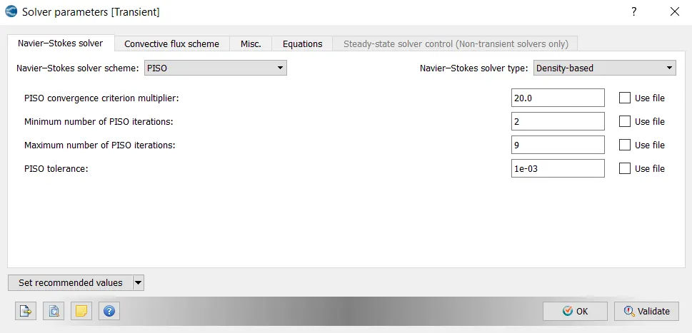
For Solver parameters, set Navier-stokes solver scheme to PISO.
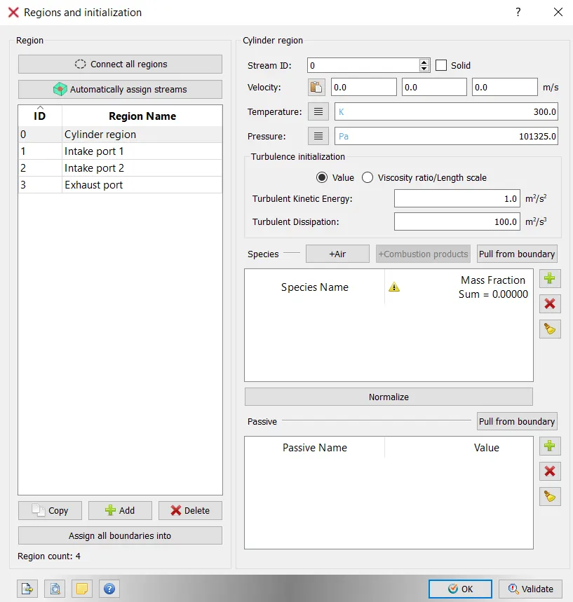
Now, regions are set up as shown in the images below.
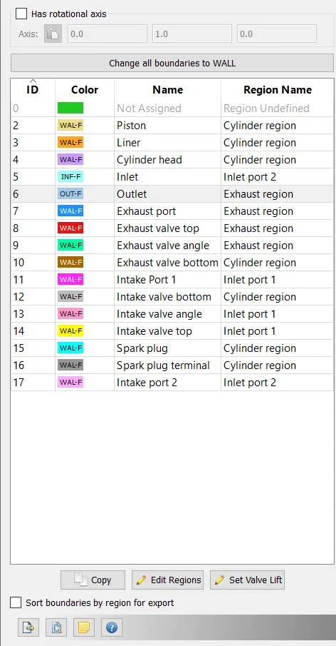
Now, the regions are assigned to the boundaries. A corresponding image is shown below.
The option of reconstruction of the boundary fences with the existing regions is used and then the geometry is grouped coloured by regions to see the regions created. A corresponding image is shown below.
4) Initial conditions and events:
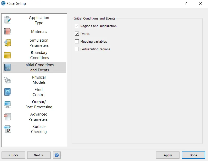
Now, under initial conditions and events, Events is checked.
i) Regions and initialization:
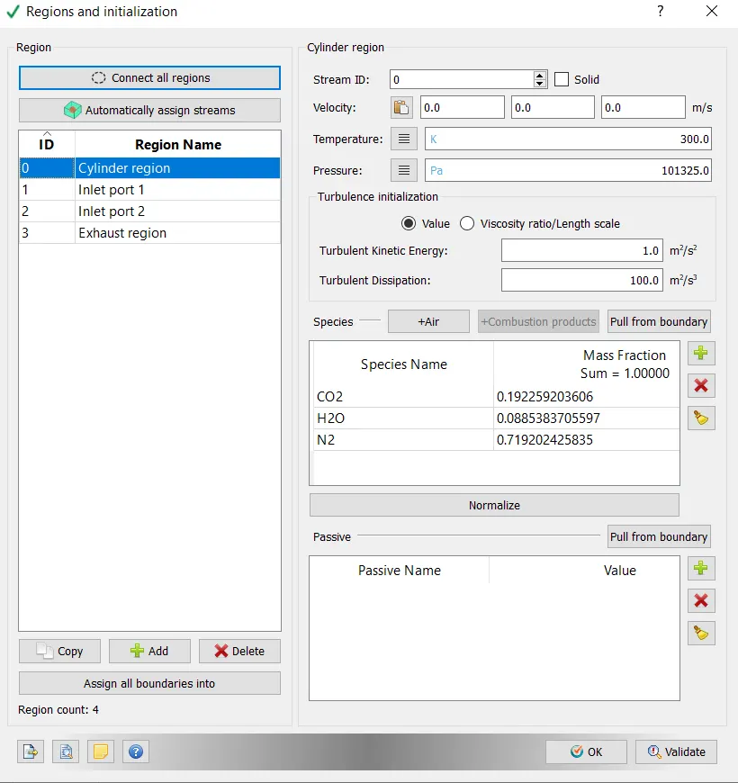
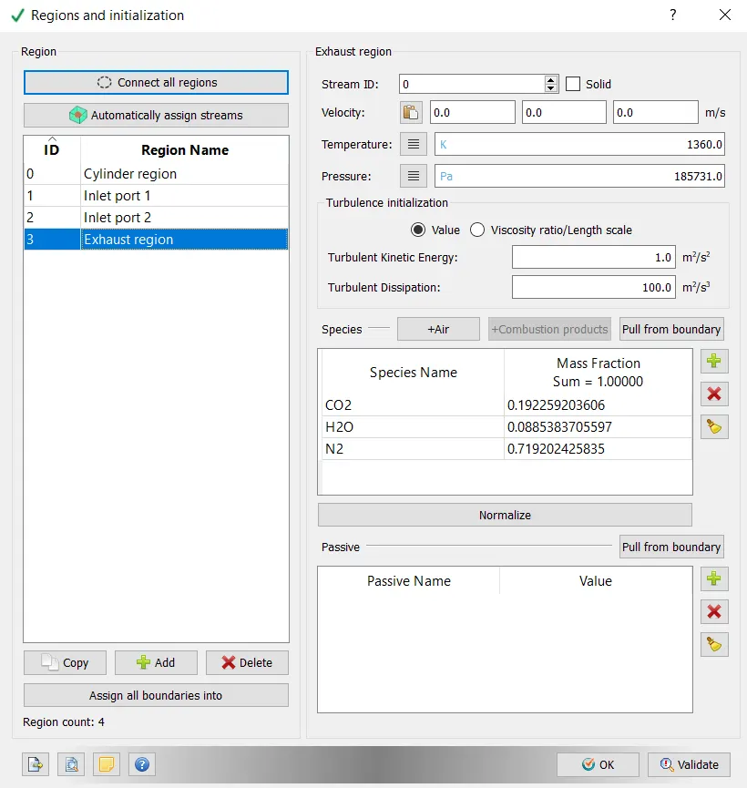
Now, the conditions for the four regions namely, Cylinder region, Inlet port 1, Inlet port 2 and Exhaust port are set.
For Cylinder region following initial conditions are set.
Temperature is set as 300 k
Pressure is set as 101325.0 Pa
Initial velocity of the species is set to 0 m/s
Species is set as follows
`CO_2` - mass fraction is 0.192259203606
`H_2O` - mass fraction is 0.0885383705597
`N_2` - mass fraction is 0719202425835
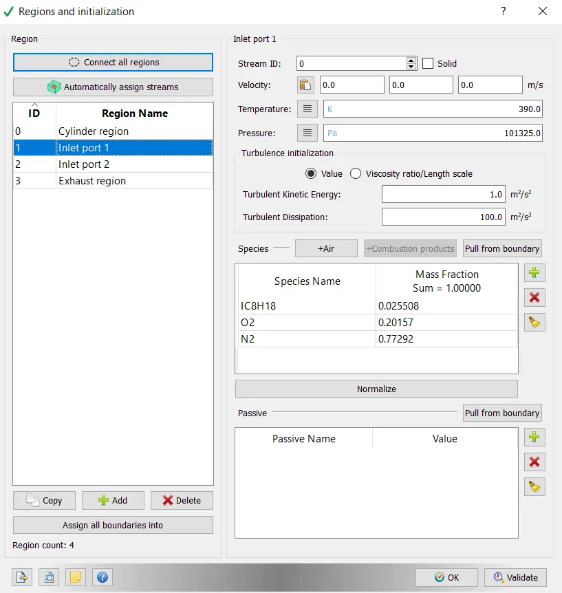
For Inlet port 1 following initial conditions are set.
Temperature is set as 390 k
Pressure is set as 101325.0 Pa
Initial velocity of the species is set to 0 m/s
Species is set as follows
`IC_8H_18` - mass fraction is 0.025508
`O_2` - mass fraction is 0.20157
`N_2` - mass fraction is 077292
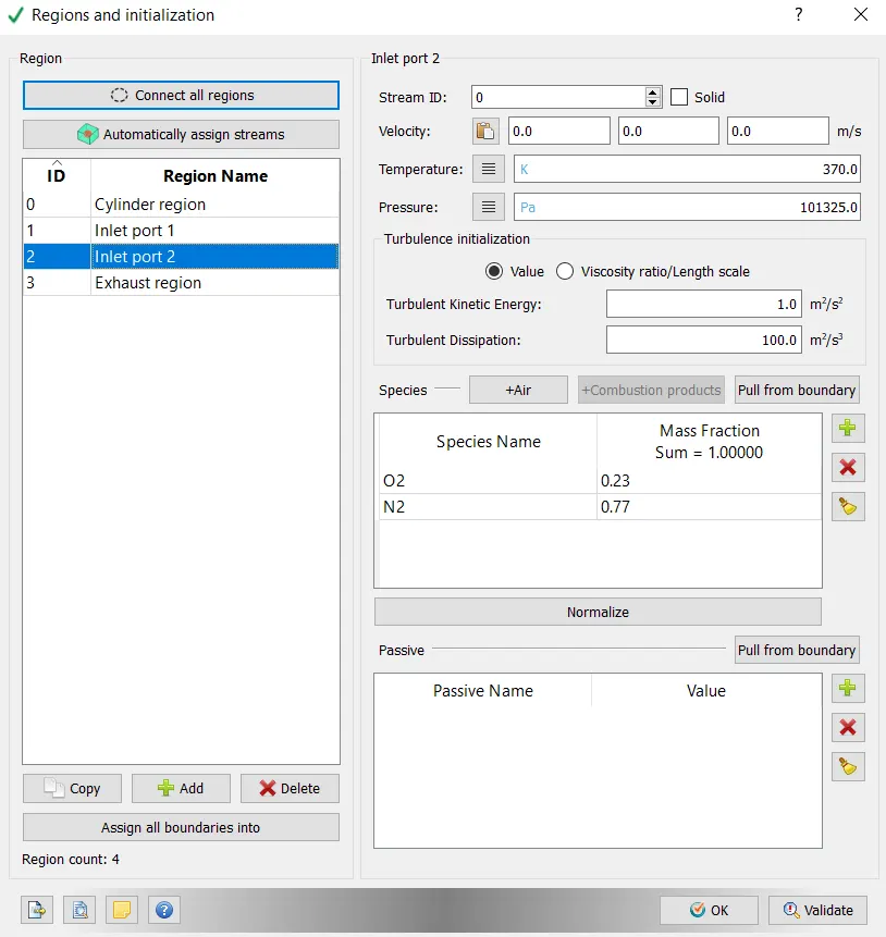
For Inlet port 2 following initial conditions are set.
Temperature is set as 370 k
Pressure is set as 101325.0 Pa
Initial velocity of the species is set to 0 m/s
Species is set as follows
`O_2` - mass fraction is 0.23
`N_2` - mass fraction is 077
For Exhaust region following initial conditions are set.
Temperature is set as 1360 k
Pressure is set as 185731.0 Pa
Initial velocity of the species is set to 0 m/s
Species is set as follows
`CO_2` - mass fraction is 0.192259203606
`H_2O` - mass fraction is 0.0885383705597
`N_2` - mass fraction is 0719202425835
ii) Events:
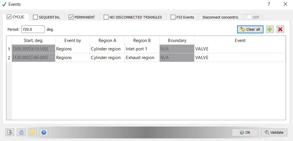
Check the cyclic events tab.
Add two events.
Event 1:
Event by: Regions
Region A: Cylinder region
Region B: Inlet port 1
Event: Valve
Event 2:
Event by: Regions
Region A: Cylinder region
Region B: Exhaust region
Event: Valve
These events are going to form disconnect triangles based on the vavle profile to control the valve motion.
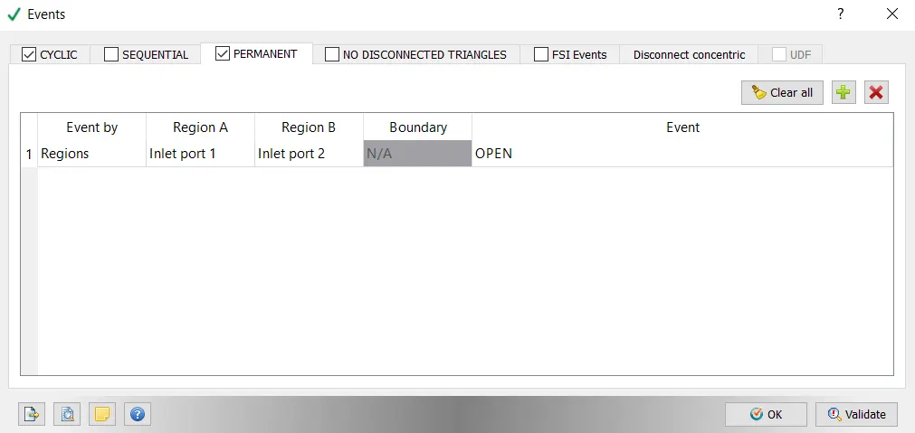
Check the permanent event tab.
Add one event.
Event:
Event by: Regions
Region A: Inlet port 1
Region B: Inlet port 2
This event allows the two regions inlet port 1 and inlet port 2 be open through out the simulation so that different initial conditions can be provided for these two regions.
5) Boundary conditions:
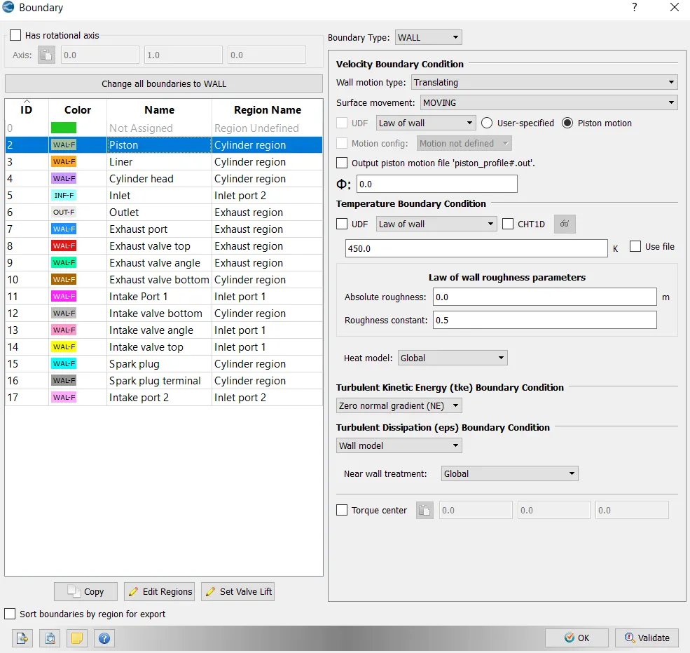
i) Piston:
For piston set the following condoitions:
Boundary type: WALL
Velocity boundary condition:
Wall motion type: Translating
Surface movement: MOVING
Wall Treatment- select 'Law of the wall' from the drop down box
Temperature boundary condition-
Select 'Law of the wall' from the drop down box. Select the Piston motion
Temperature value- 450.0 k
Turbulent Kinetic energy boundary Condition-
Zero normal gradient (NE)
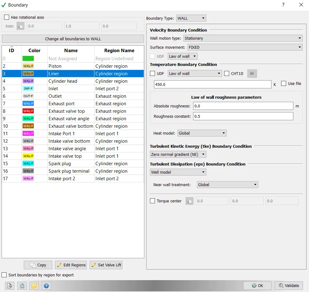
ii) Liner:
For liner set the following condoitions:
Boundary type: WALL
Velocity boundary condition:
Wall motion type: stationary
Surface movement: FIXED
Wall Treatment- select 'Law of the wall' from the drop down box
Temperature boundary condition-
Select 'Law of the wall' from the drop down box.
Temperature value- 450.0 k
Turbulent Kinetic energy boundary Condition-
Zero normal gradient (NE)
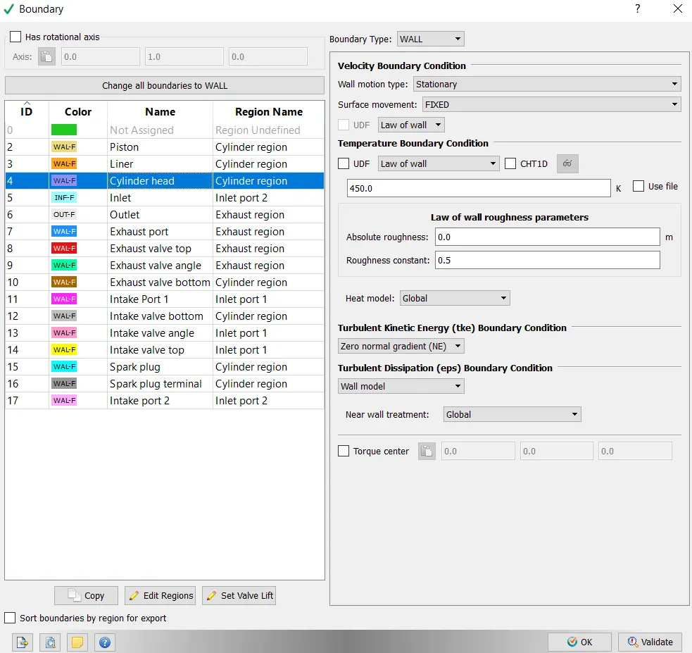
iii) Cylinder head:
For Cylinder head set the following condoitions:
Boundary type: WALL
Velocity boundary condition:
Wall motion type: Stationary
Surface movement: FIXED
Wall Treatment- select 'Law of the wall' from the drop down box
Temperature boundary condition-
Select 'Law of the wall' from the drop down box.
Temperature value- 450.0 k
Turbulent Kinetic energy boundary Condition-
Zero normal gradient (NE)
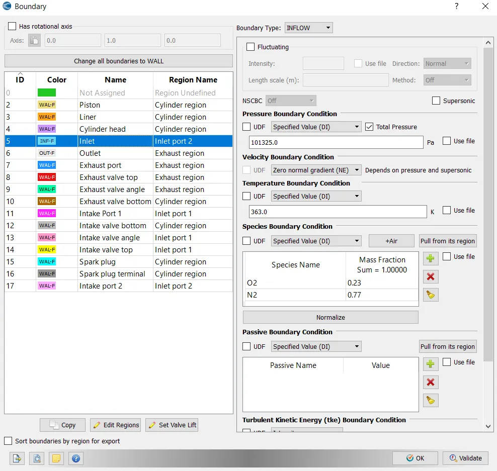
iv) Inlet:
For Inlet boundary following conditions are set.
Boundary type: INFLOW
Pressure boundary condition:
Specified value (DI) is selected from the drop down box.
pressure value: 101325.0 Pa
Velocity boundary condition:
Zero Normal Gradient (NE) is selected from the drop down box.
Temperature boundary condition:
Specified value (DI) is selected from the drop down box.
Temperature value: 363.0 k
Species is set as follows
`O_2` - mass fraction is 0.23
`N_2` - mass fraction is 077.
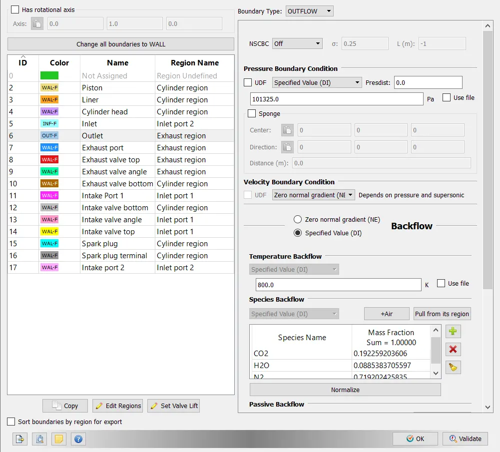
v) Outlet:
For Outlet boundary following conditions are set.
Boundary type: OUTFLOW
Pressure boundary condition:
Specified value (DI) is selected from the drop down box.
pressure value: 101325.0 Pa
Velocity boundary condition:
Zero Normal Gradient (NE) is selected from the drop down box.
Backflow:
Temperature backflow: 800.0 k
Species : Pull from its region option is selected.
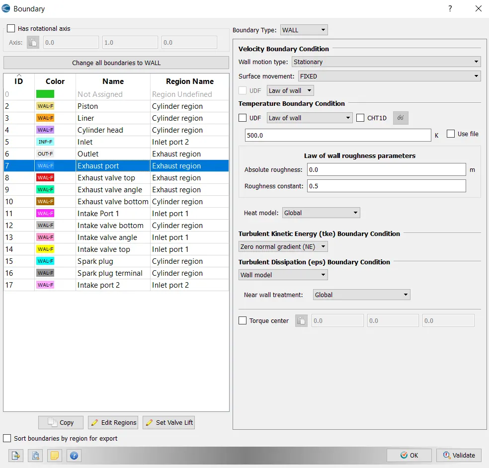
vi) Exhaust port:
For Exhaust port set the following condoitions:
Boundary type: WALL
Velocity boundary condition:
Wall motion type: Stationary
Surface movement: FIXED
Wall Treatment- select 'Law of the wall' from the drop down box
Temperature boundary condition-
Select 'Law of the wall' from the drop down box.
Temperature value- 500.0 k
Turbulent Kinetic energy boundary Condition-
Zero normal gradient (NE)
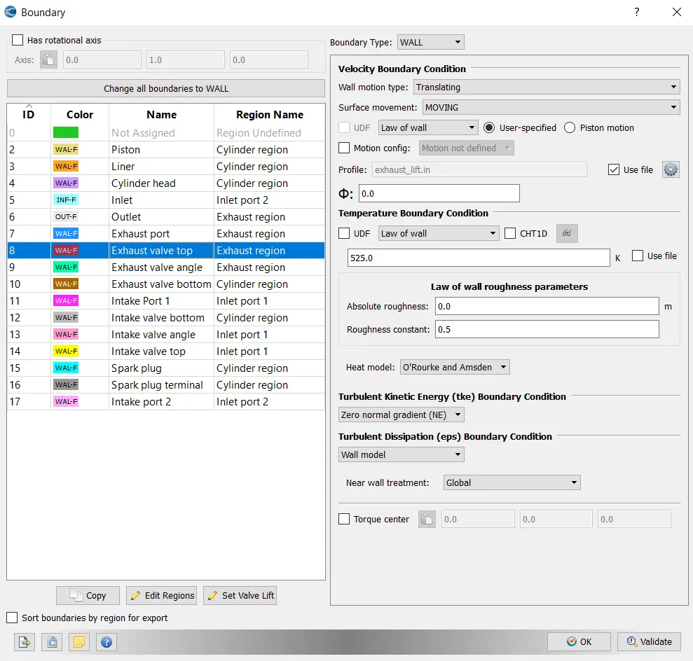
vii) Exhaust valve top:
For Exhaust valve top set the following condoitions:
Boundary type: WALL
Velocity boundary condition:
Wall motion type: Translating
Surface movement: MOVING
Wall Treatment- select 'Law of the wall' from the drop down box.
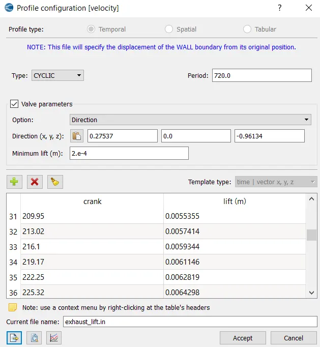
Profile: A file exhaust_lift.in is used and the minimum lift is set as 2e-4m
Temperature boundary condition-
Select 'Law of the wall' from the drop down box.
Temperature value- 525.0 k
Turbulent Kinetic energy boundary Condition-
Zero normal gradient (NE)
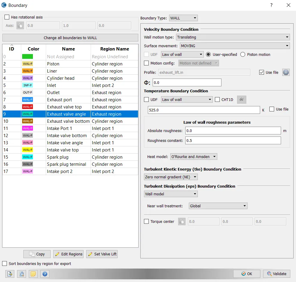
viii) Exhaust valve angle:
For Exhaust valve angle set the following condoitions:
Boundary type: WALL
Velocity boundary condition:
Wall motion type: Translating
Surface movement: MOVING
Wall Treatment- select 'Law of the wall' from the drop down box.
Profile: A file exhaust_lift.in is used and the minimum lift is set as 2e-4m
Temperature boundary condition-
Select 'Law of the wall' from the drop down box.
Temperature value- 525.0 k
Turbulent Kinetic energy boundary Condition-
Zero normal gradient (NE)
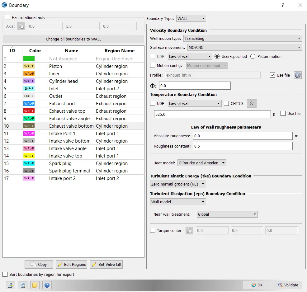
ix) Exhaust valve bottom:
For Exhaust valve bottom set the following condoitions:
Boundary type: WALL
Velocity boundary condition:
Wall motion type: Translating
Surface movement: MOVING
Wall Treatment- select 'Law of the wall' from the drop down box.
Profile: A file exhaust_lift.in is used and the minimum lift is set as 2e-4m
Temperature boundary condition-
Select 'Law of the wall' from the drop down box.
Temperature value- 525.0 k
Turbulent Kinetic energy boundary Condition-
Zero normal gradient (NE)
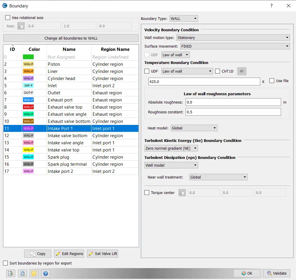
x) Intake port 1:
For Intake port 1 set the following condoitions:
Boundary type: WALL
Velocity boundary condition:
Wall motion type: Stationary
Surface movement: FIXED
Wall Treatment- select 'Law of the wall' from the drop down box
Temperature boundary condition-
Select 'Law of the wall' from the drop down box.
Temperature value- 425.0 k
Turbulent Kinetic energy boundary Condition-
Zero normal gradient (NE)
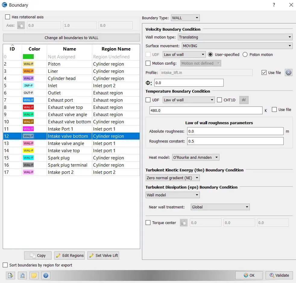
xi) Intake valve bottom:
For Intake valve bottom set the following condoitions:
Boundary type: WALL
Velocity boundary condition:
Wall motion type: Translating
Surface movement: MOVING
Wall Treatment- select 'Law of the wall' from the drop down box.
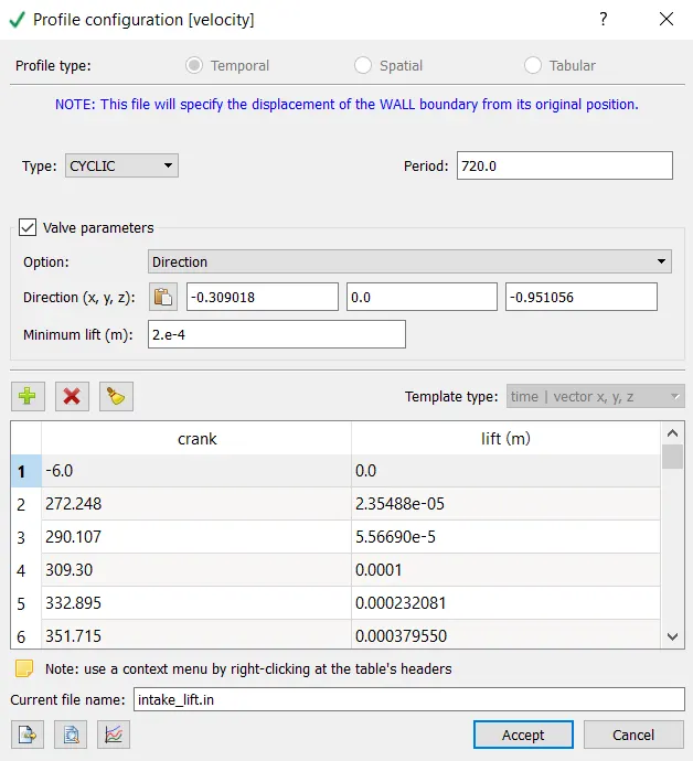
Profile: A file intake_lift.in is used.
Temperature boundary condition-
Select 'Law of the wall' from the drop down box.
Temperature value- 480.0 k
Turbulent Kinetic energy boundary Condition-
Zero normal gradient (NE)
xii) Intake valve angle:
For Intake valve angle set the following condoitions:
Boundary type: WALL
Velocity boundary condition:
Wall motion type: Translating
Surface movement: MOVING
Wall Treatment- select 'Law of the wall' from the drop down box.
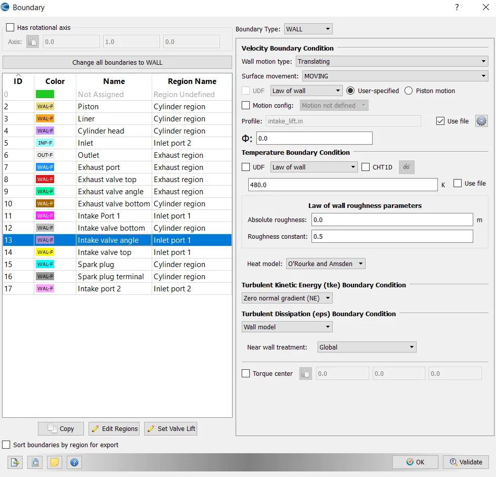
Profile: A file intake_lift.in is used.
Temperature boundary condition-
Select 'Law of the wall' from the drop down box.
Temperature value- 480.0 k
Turbulent Kinetic energy boundary Condition-
Zero normal gradient (NE)
xiii) Intake valve top:
For Intake valve top set the following condoitions:
Boundary type: WALL
Velocity boundary condition:
Wall motion type: Translating
Surface movement: MOVING
Wall Treatment- select 'Law of the wall' from the drop down box.
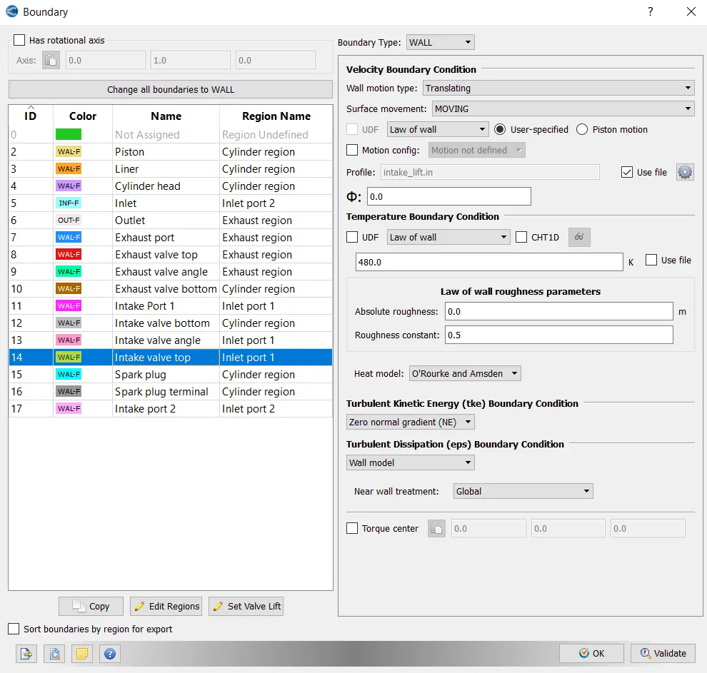
Profile: A file intake_lift.in is used.
Temperature boundary condition-
Select 'Law of the wall' from the drop down box.
Temperature value- 480.0 k
Turbulent Kinetic energy boundary Condition-
Zero normal gradient (NE)
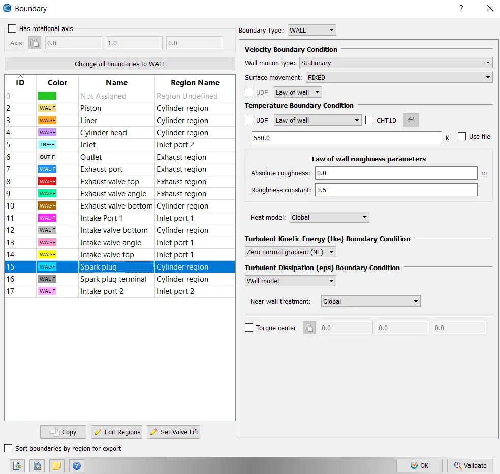
xiv) Spark plug:
For Spark plug set the following condoitions:
Boundary type: WALL
Velocity boundary condition:
Wall motion type: Stationary
Surface movement: FIXED
Wall Treatment- select 'Law of the wall' from the drop down box
Temperature boundary condition-
Select 'Law of the wall' from the drop down box.
Temperature value- 550.0 k
Turbulent Kinetic energy boundary Condition-
Zero normal gradient (NE)
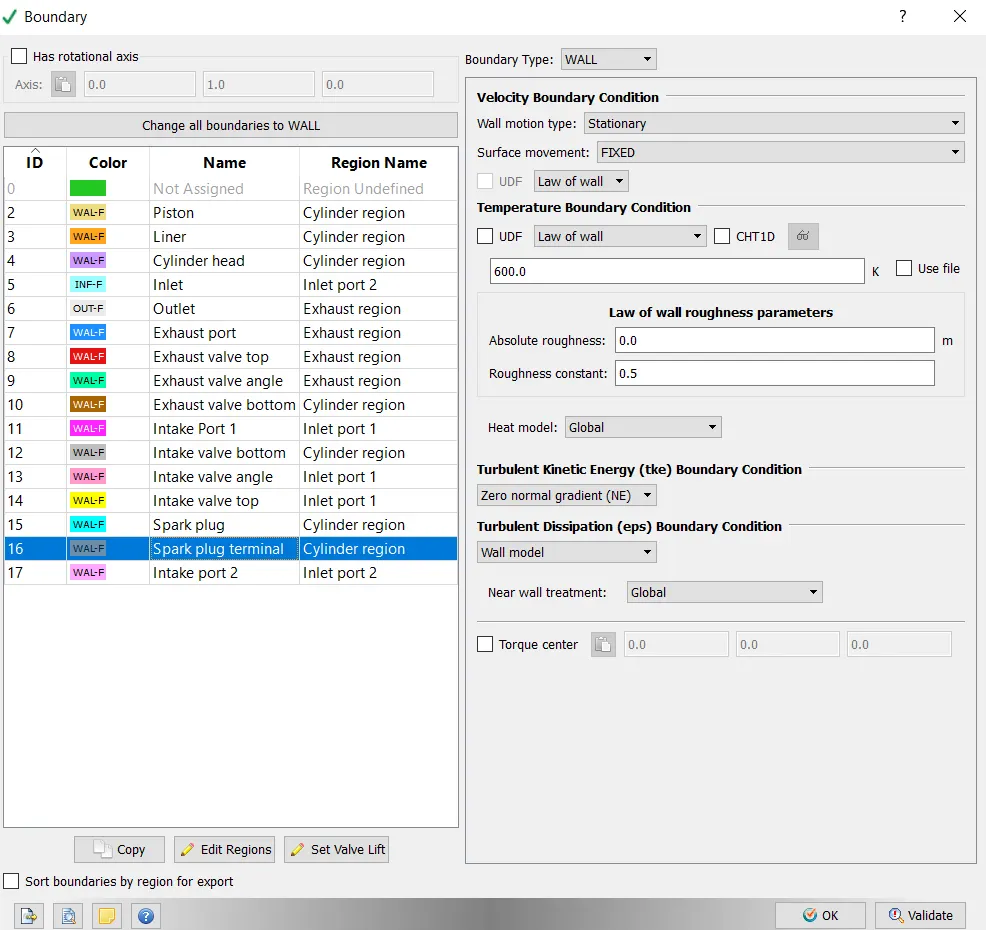
xv) Spark plug terminal:
For Spark plug terminal set the following condoitions:
Boundary type: WALL
Velocity boundary condition:
Wall motion type: Stationary
Surface movement: FIXED
Wall Treatment- select 'Law of the wall' from the drop down box
Temperature boundary condition-
Select 'Law of the wall' from the drop down box.
Temperature value- 600.0 k
Turbulent Kinetic energy boundary Condition-
Zero normal gradient (NE)
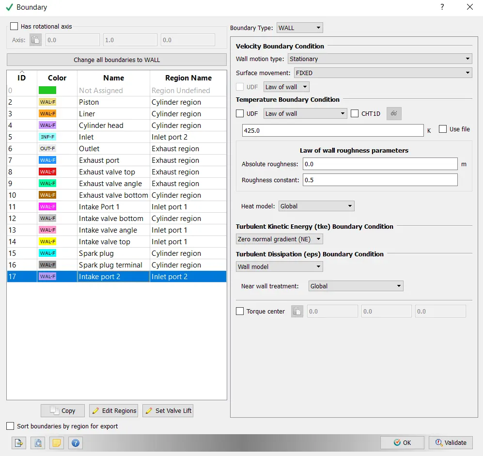
xvi) Intake port 2:
For Intake port 2 set the following condoitions:
Boundary type: WALL
Velocity boundary condition:
Wall motion type: Stationary
Surface movement: FIXED
Wall Treatment- select 'Law of the wall' from the drop down box
Temperature boundary condition-
Select 'Law of the wall' from the drop down box.
Temperature value- 425.0 k
Turbulent Kinetic energy boundary Condition-
Zero normal gradient (NE)
6) Physical models:
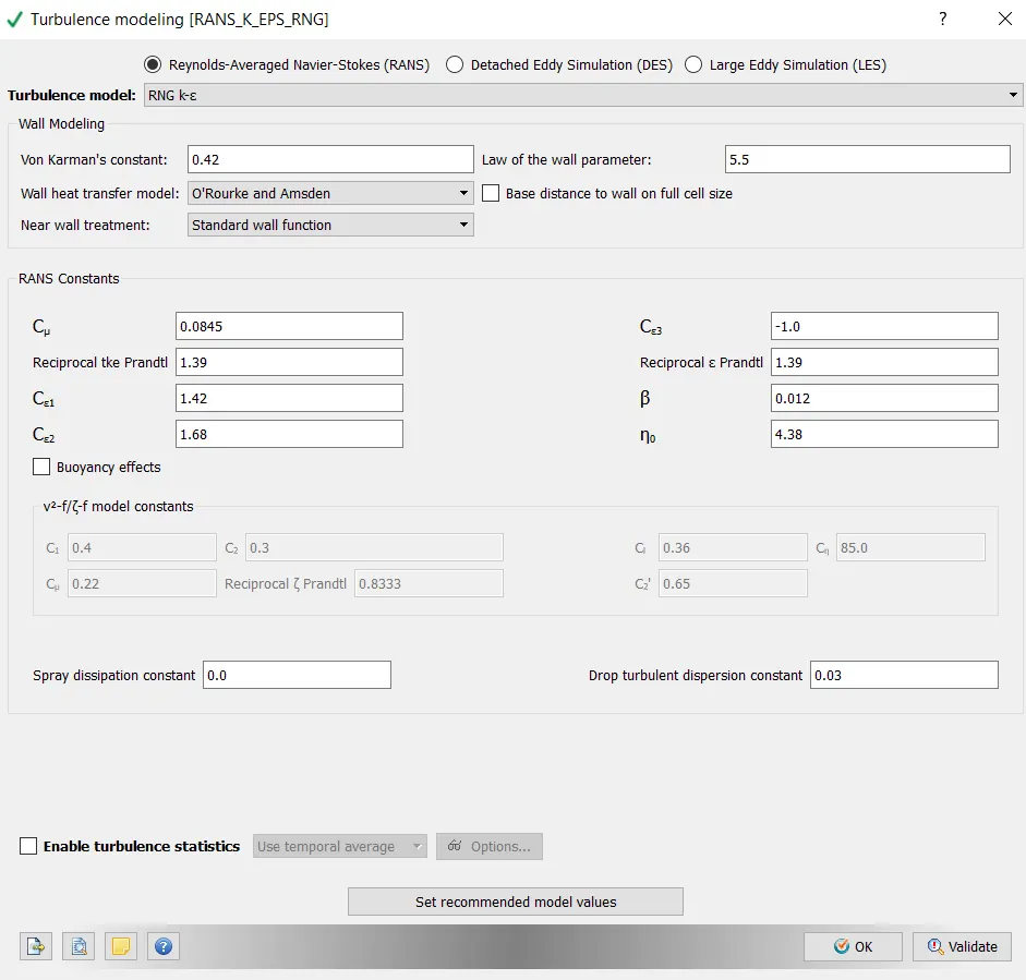
Turbulence modelling:
For turbulence modelling select the following:
Turbulence model: RNG k-epsilon
Remaining parameters are set as default.
7) Grid control:
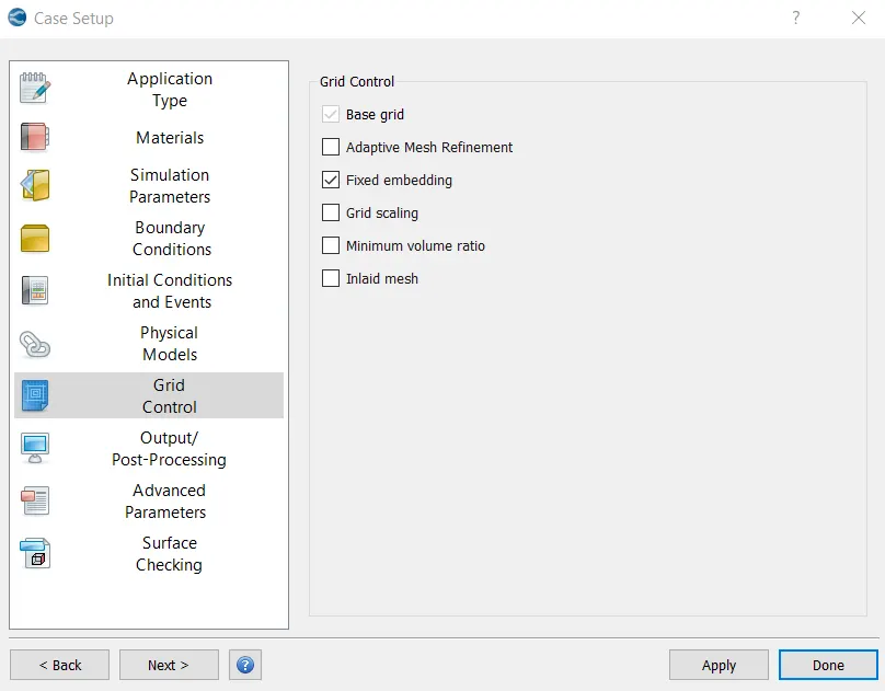
In grid control, check fixed embedding.
i) Base grid:
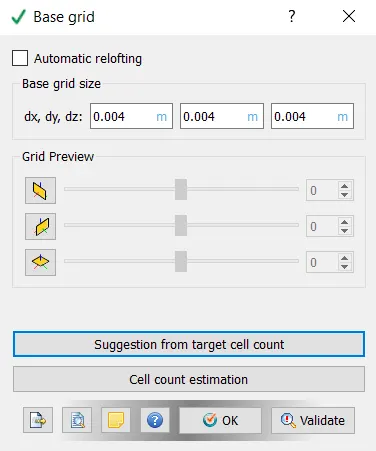
Set base grid as dx=dy=dz=0.004 m
ii) Fixed embedding:
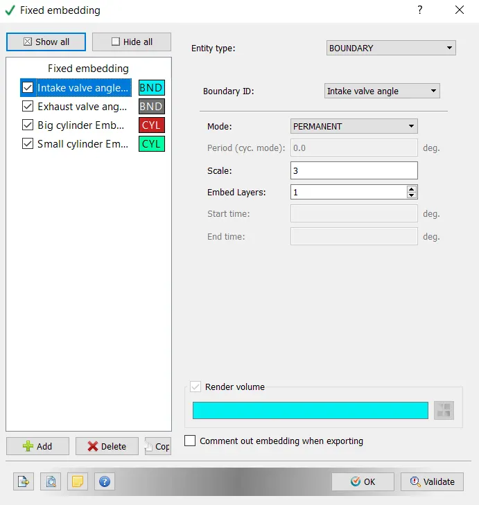
Add four fixed embedding namely, Intake valve angle embedding, Exhaust valve angle embedding, Big cylinder embedding and Small cylinder embedding.
a) Intake valve angle embedding:
This is done to make finer mesh at intake valve angle boundary without meeting the conditions of cell pairing.
The settings of this embedding are as follows:
Entity type: BOUNDARY
Boundary ID: Intake valve angle
Mode: PERMANENT
Scale: 3
Embed Layers: 1
b) Exhaust valve angle embedding:
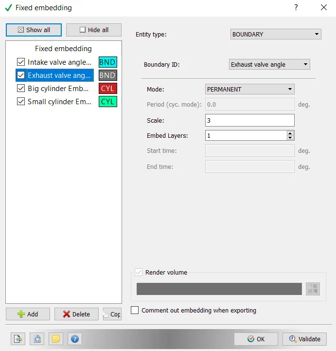
Similarly the exhaust valve angle embedding is done with the following settings:
Entity type: BOUNDARY
Boundary ID: Exhaust valve angle
Mode: PERMANENT
Scale: 3
Embed Layers: 1
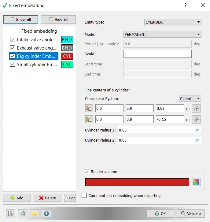
c) Big cylinder embedding:
This embedding is done so that a finer mesh size can be obtained for liner boundary, cylinder head and valve bottom and angle and top boundary. The amount of embedding should be done in such a way that it should not have huge number of cells and also that the cells should capture reasonable amount of data during the simulation.
The settings of this embedding are as follows:
Entity type: CYLINDER
Mode: PERMANENT
Scale: 1
Centers of the cylinder are selected in such a way that the liner boundary, cylinder head and valve bottom, angle and top boundaries are under this cylinder.
centre 1: (0.0m, 0.0m, 0.08m)
Centre 2: ( 0.0m, 0.0m, -0.15m)
d) Small cylinder embedding:
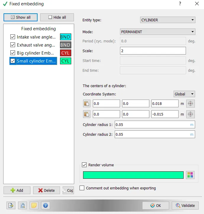
This embedding is done in such a way that more finer mesh is obtained in the boundaries of Cylinder head, Valve bottom and angle.
The settings of this embedding are as follows:
Entity type: CYLINDER
Mode: PERMANENT
Scale: 2
Centers of the cylinder are selected in such a way that cylinder head and valve bottom, angle and top boundaries are under this cylinder.
centre 1: (0.0m, 0.0m, 0.08m)
Centre 2: ( 0.0m, 0.0m, -0.015m)
8) Output/Post-processing:
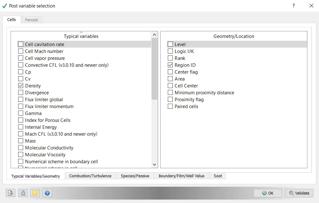
i) Post variable selection: This is set as default as this is a No hydro simulation.
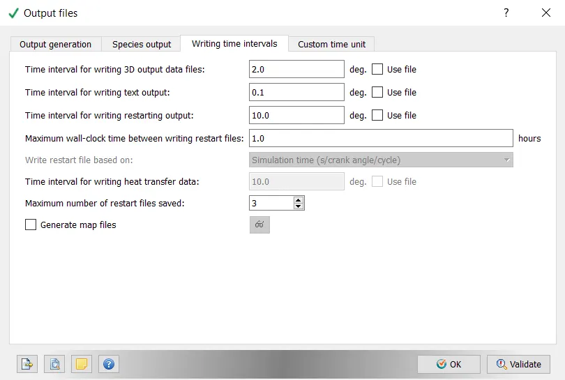
ii) Output files: These are also set as default.
The next step after setting up the case is to process the inputs in a solver such as Cygwin terminal. The input files of this case setup are exported and the solver processes them. After this, the results are post processed in a software called Paraview or Ensight.
Results:
The link for mesh generation animation in 2D is shown below:
In the above animation the inlet valve is on the right hand side of the screen. Mesh generation at different parts of the PFI engine is different because of fixed embedding done in the grid control.
The link for the no hydro simulation in 3D is shown below:
In the above animation the piston motion and the valve motion can be seen for one complete cycle which is four strokes of the piston or 720 degrees crank angle.
Conclusion:
The surface preparation and boundary flagging of a PFI Engine is completed successfully.
No hydro simulaltion is also simulated and the mesh generated is found to have no errors.