Study of Channel Flow using Converge Studio

STUDYING THE CHANNEL FLOW USING CONVERGE STUDIO

Channel flow, a branch of hydraulics and fluid mechanics, is a type of fluid flow within a channel. There are two type of channel flow one is open channel flow and the other is closed/conduit channel flow. These two type of clow are similar in many ways, but differ in one important aspect. Pipe flow do not have a free surface which is found in open-channel flow. Pipe flow, being confined within closed conduit, does not exert direct atmospheric pressure, but does exert hydraulic pressure on the conduit.

A conduit is any pipe,tube, or duct that is completely filled with a flowing fluid. Examples include a pipeline transporting liquified natural gas, a microchannel transporting hydrogen in a fuel cell, and a duct transporting air for heating of a building.

Flow in closed conduits (pipe, if conduit is circular in section, and duct otherwise) differs from that of open channel flow in the mechanism that derives the flow. In the case of open channel flow, flow occurs due to the action of gravity.

In closed conduit flow, however, although gravity is important, the main driving force is the pressure gradient along the flow.

The emphsis of this project is on ducts. Flow in Ducts is an example of internal flow, i.e., the flow is bounded by the walls, in contrast to external flow where the flow is unbounded.

Methodlogy

A simplified model of duct was modeled to represent the real Duct present in the industry. The model contain the wall, velocity inlet, outlet. A monitoring plane was used to observe the velocity contour inside the duct.

To simulate all these phenomenon we have used Converge CFD which is a commercial software. Converge is a computational code that allows the user to simulate the real physics of phenomenon and substantially reduce the expensive remort machine.

Geometry Configuration

The dimension can be seen in the diagram-

l_x= 0.1 meter

l_y= 0.01 meter

l_z= 0.01 meter

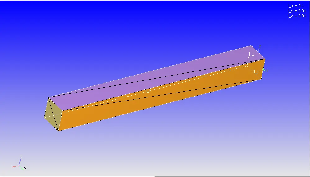
Fig1. Geometry

Fig2- Boundary of the geometry

Mathematical modelling

Any physical phenomenon can be represented as a mathematical model that gives us the information about the processes that is going on the domain. These mathematical modelling basically represent the information about the behaviour of the process through governing equations.

Governing equation consist of partial differential equation-

1. Continuity equation

`(delP)/(delt)+(del(rhou))/(delx)+(del(rhov))/(dely)+(del(rhow))/(delz)=0`

2. Momentum Conservation

`(del(rhou))/(delt)+(del(rhou u))/(delx)+(del(rhovu))/(dely)+(del(rhowu))/(delz)= (del(Px x))/(delx)+(del(Pyx))/(dely)+(del(Pzx))/(delz)` X momentum equation

`(del(rhov))/(delt)+(del(rhouv))/(delx)+(del(rhov v))/(dely)+(del(rhowv))/(delz)= (del(Pxy))/(delx)+(del(Py y))/(dely)+(del(Pzy))/(delz)` Y momentum equation

`(del(rhow))/(delt)+(del(rhou w))/(delx)+(del(rhovw))/(dely)+(del(rhoww))/(delz)= (del(Pxz))/(delx)+(del(Pyz))/(dely)+(del(Pz z))/(delz)` Z momentum equation

3. Energy Conservation

`(delE)/(delt)+(del(uui*E-uuj*P ij+Qi))/(dxi)=0`

Here `rho` is the mass density, `uuij` is the velocity, `E` is the energy density, `P ij` is the stress tensor, `Qi` is the heat flux. `i,j,k` are the stress indices and varies from 1 to 3. Repeated indices indicates that it is summed over 1 to 3.

The stress tensor and energy density are-

`P ij=-nKTdeltaij-2/3*mu(deluuk)/(delxk)*deltaij+mu((deluui)/(delxj)+(deluuj)/(delx i))`

`E=3/2nkT+1/2rhouu^2`

Where the density `n=rho/m`, m is mass and T is the temperature. The heat flux `Q` is approximated by Fourier's law `Q=-knablaT`.

This 3 form of equation are termed as Naviers Stokes equation. In addition to that we have one more equation to be solved and that is called species transport equation because we are simulating air in the domain-

4. Species Conservation equation

`(delrhomi)/(delt)+grad*(rhoumi+J)=R`

where `mi` is the mass fraction of the ith species and R is the source term that accounts for any species generation.

Boundary Conditions

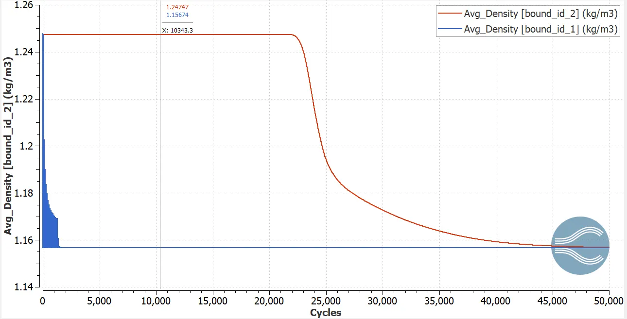
The air is assumed as steady flow and compressible throughout the flow and we can find out by post processing our results that how the density is changing through the time.

The temperature of the air is assumed to be same as the room temperature 300 k.

The pressure of the air at the inlet is assumed as ideal atmospheric pressure, 100001 Pa as a static pressure because we dont know till now about the velocity there so we cant say about the dynamic pressure at inlet. The top and bottom wall is taken as wall boundary conditions and front and back is taken as 2D symmetry condition.

The pressure at the outlet is 100000 pa and considered at atmospheric pressure.

The type of flow is modeled as compressible flow because the fluid is air(oxygen+nitrogen) here. The air is modeled as Laminar as the Reynolds number achieves Turbulent criteria for internal flow (Re < 4000). This is because only 1 pascal pressure difference can't generate a large velocity gradient in the domain in x direction. Thus the turbulent model is off here.

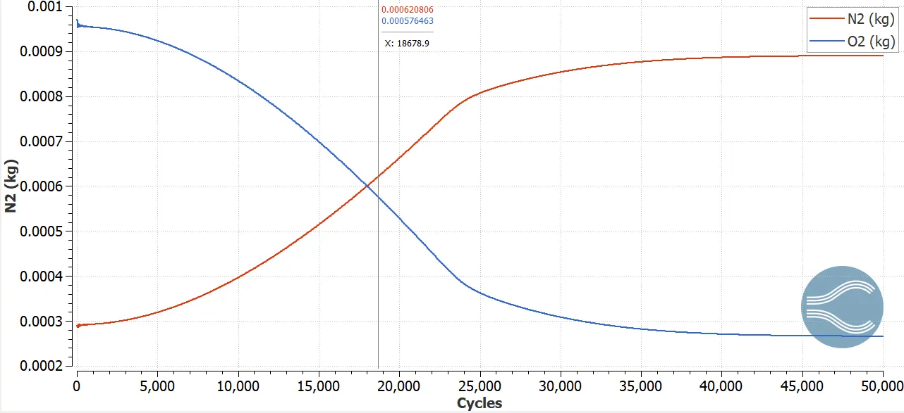
Initial mass fraction of O2 and N2 are 0.77 and 0.23 respectively. All these arrangement was solved by a steady state PISO solver.

Case Study

We have simulated the geometry for three different mesh sizes-

dimension	mesh1	mesh2	mesh3
dx	2e-4	1.5e-4	2e-4
dy	2e-4	1.5e-4	1.5e-4
dz	2e-4	1.0e-4	1.0e-4

Mesh1

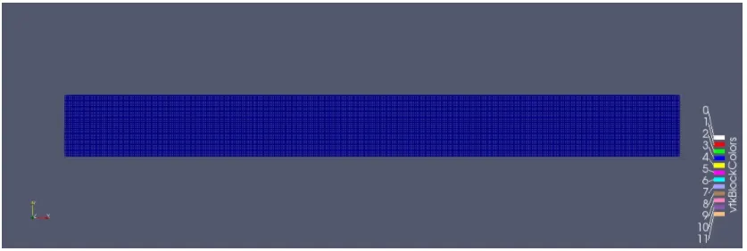
Fig3- Cartesian mesh of the domain

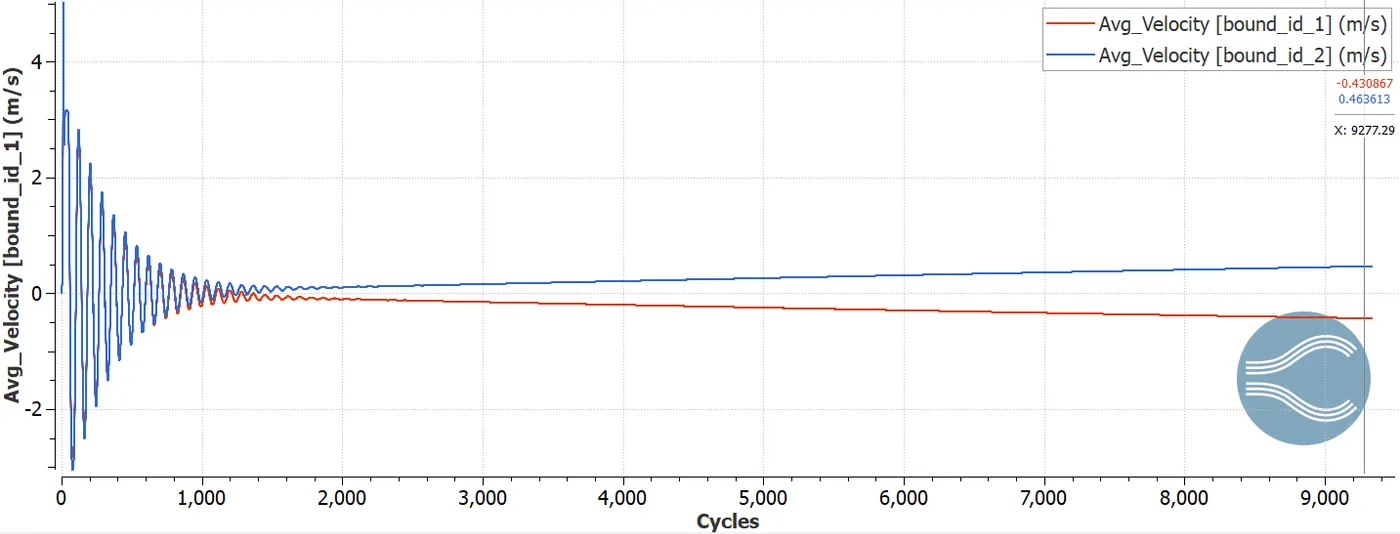
Fig4- Avg velocity at inlegt and outlet

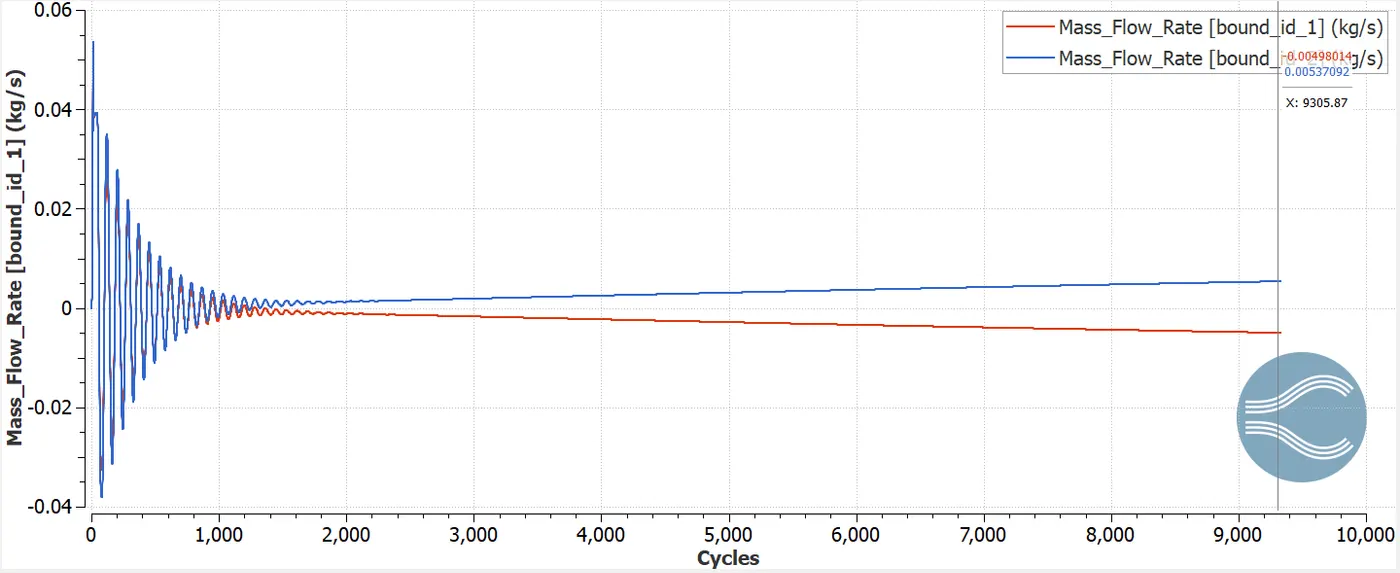
Fig5- Mass Flow rate at inlet and outlet

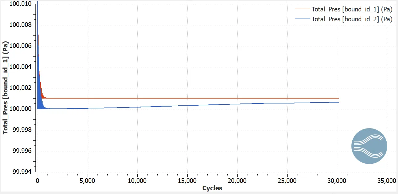
Fig6- Pressure at the inlet and outlet

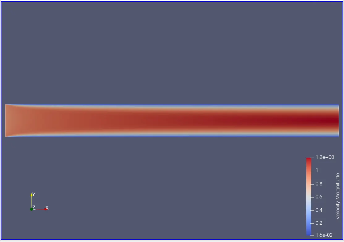
Fig7- Velocity contour in the domain

Velocity Animation (mesh1)

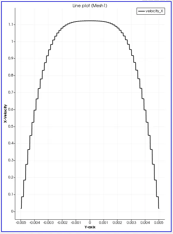
velocity gradient along y axix

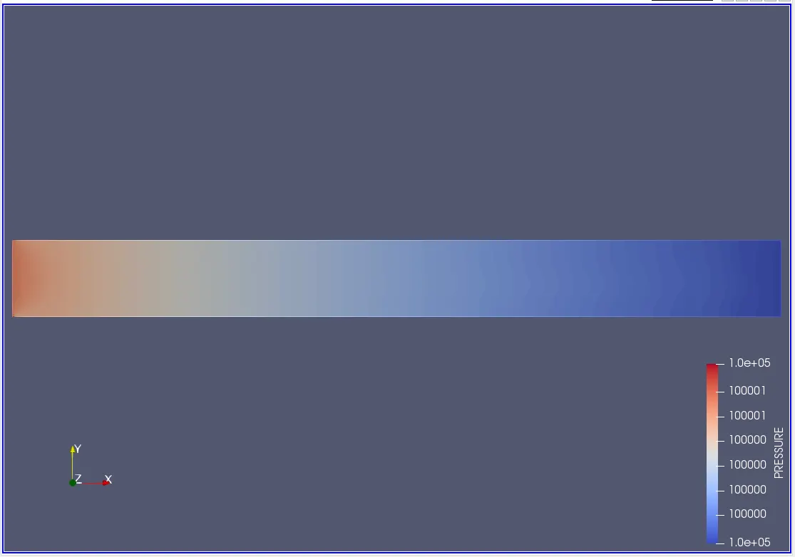
Fig8- Pressure Contour in domain

cell count= 26000

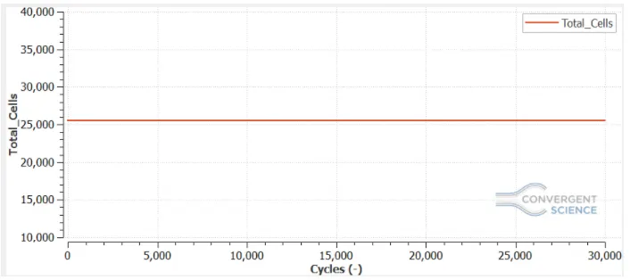
Fig9- Total cell count in the domain

Mesh2

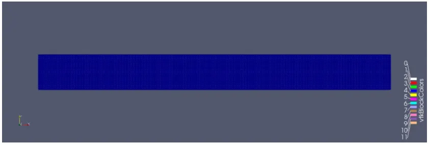
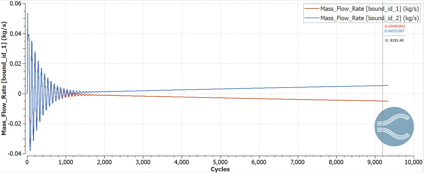
Fig10- Mass flow rate at the inlet and outlet

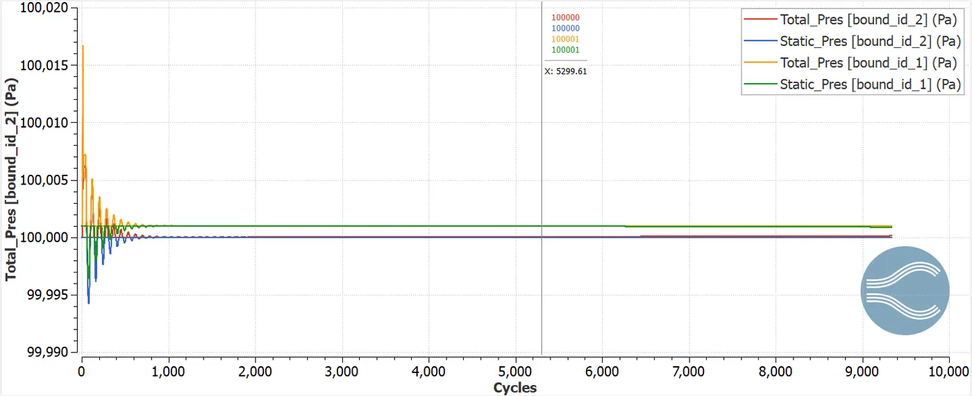
Fig11- Pressre plot at the inlet and outlet

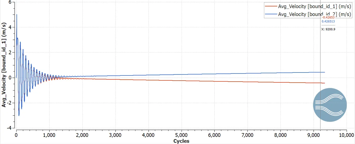
Fig12- Average velocity at the inlet and the outlet

cell counts= 45420

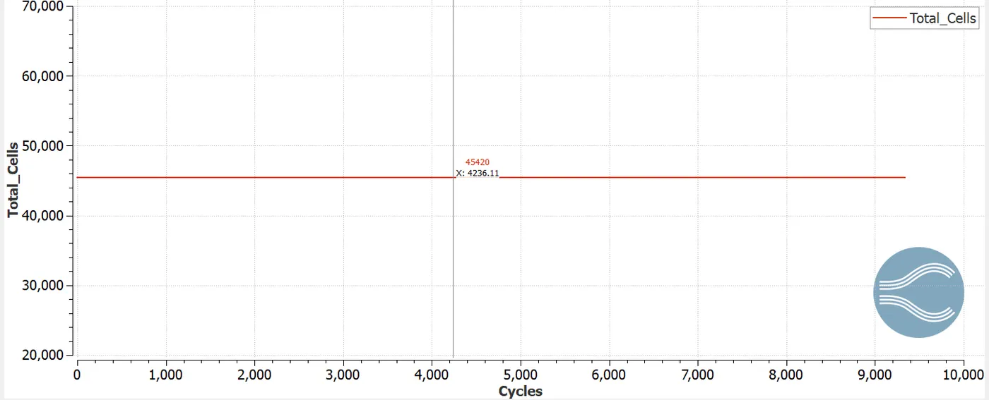
Fig13- Total cell counts

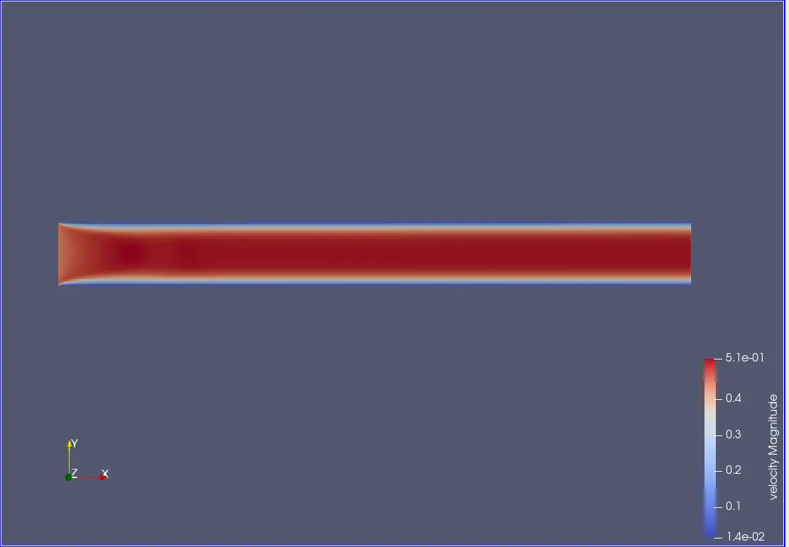
Fig14- Velocity contour of the domain

Velocity animation of mesh2

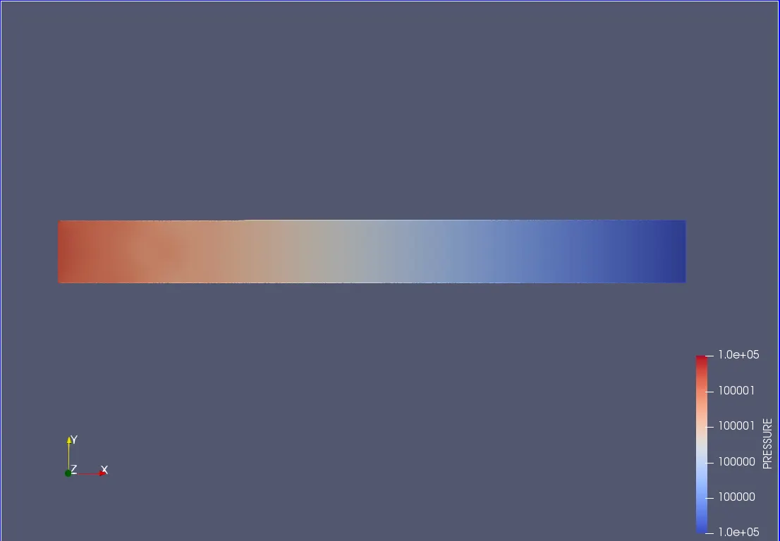
Fig15- Pressure Contour of the domain

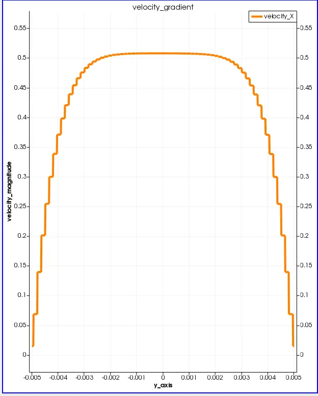Fig16- Velocity gradient profile

Mesh3

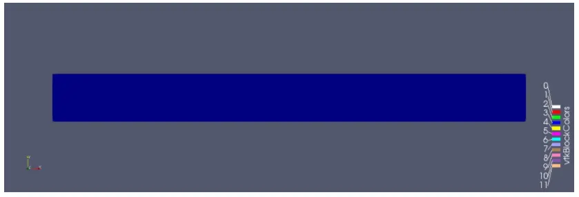
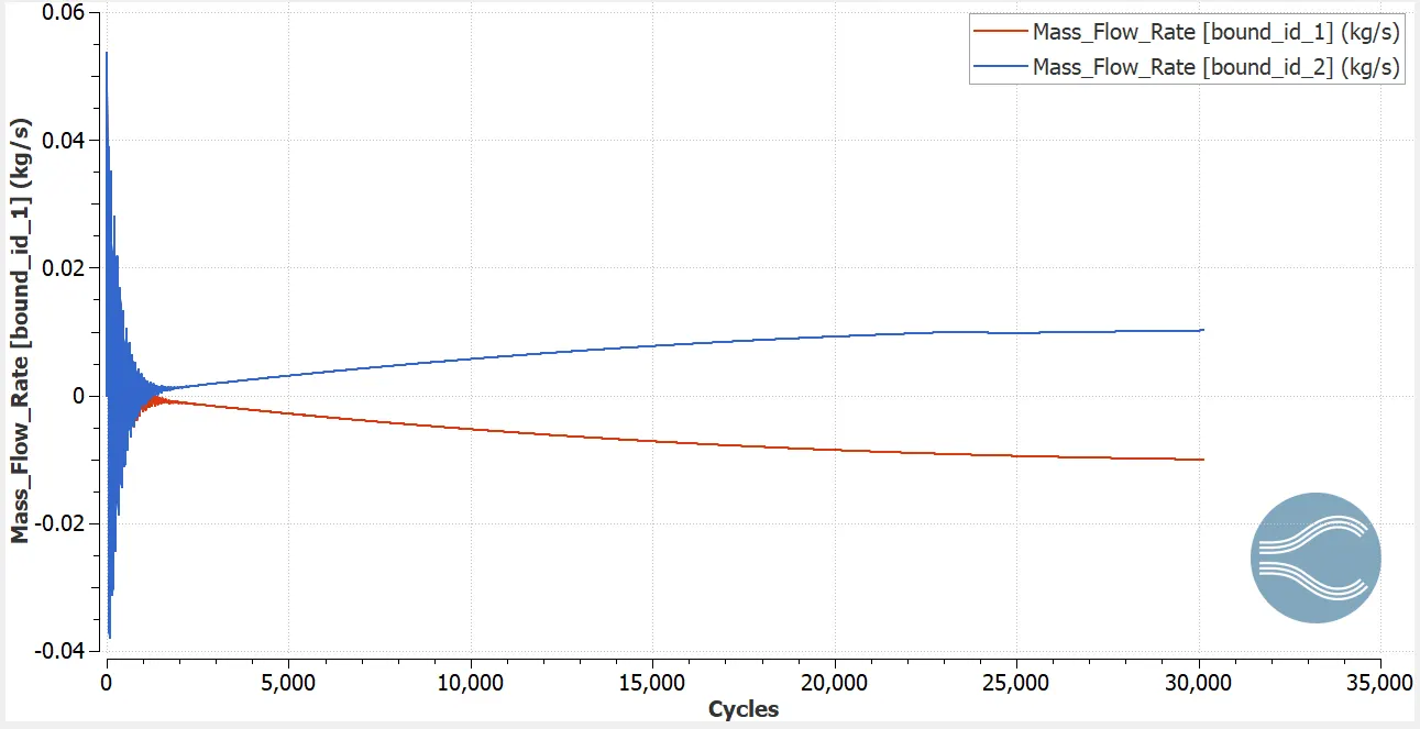
Fig14- Mass average flow rate at inlet and outlet

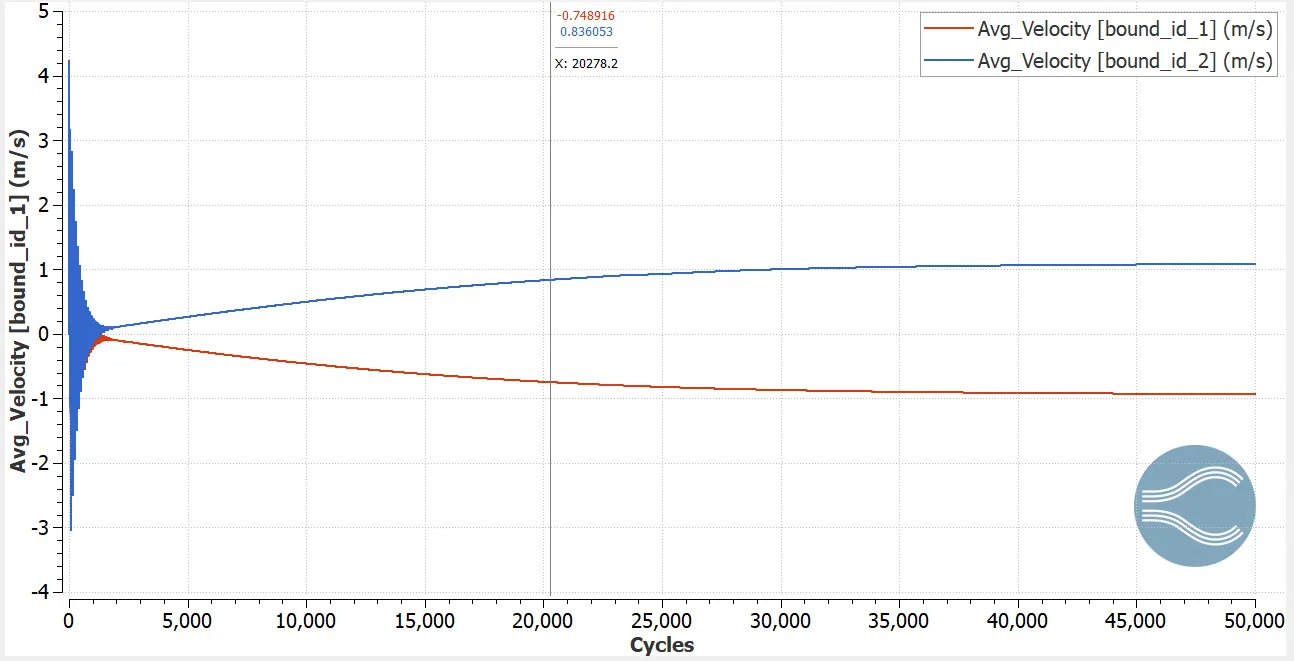
Fig17- Average velocity at inlet and outlet

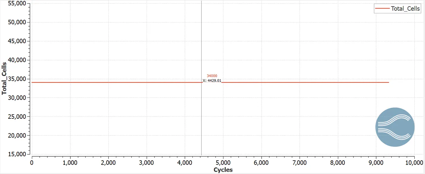
Fig18- Total cell counts

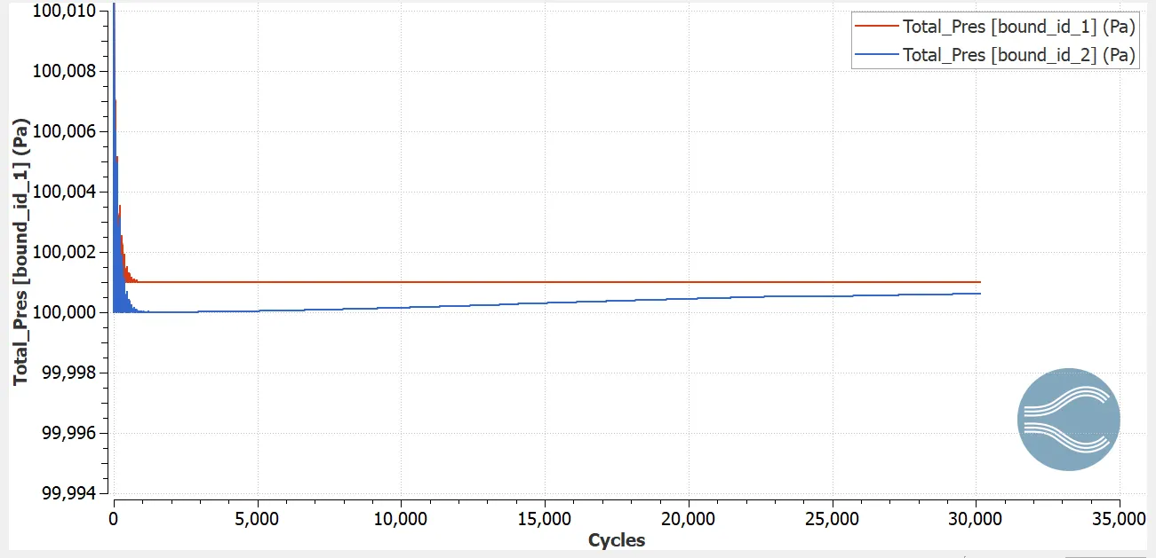
Fig19. Total pressure ate inlet and outlet

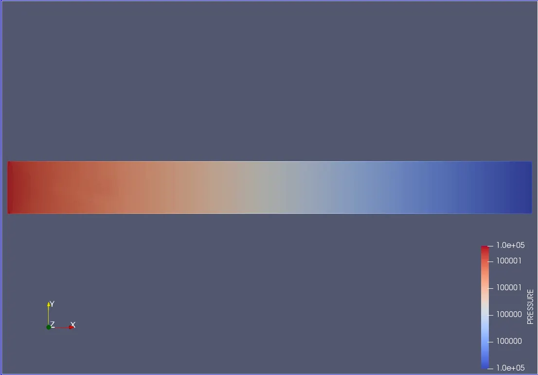
Fig19- Pressure contour of the domain

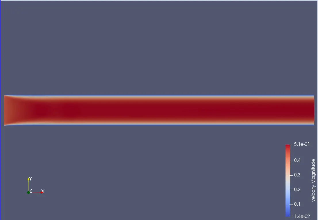
Fig20- Velocity contour of the domain

Animation of velocity (mesh3)

Important Findings and Conclusions

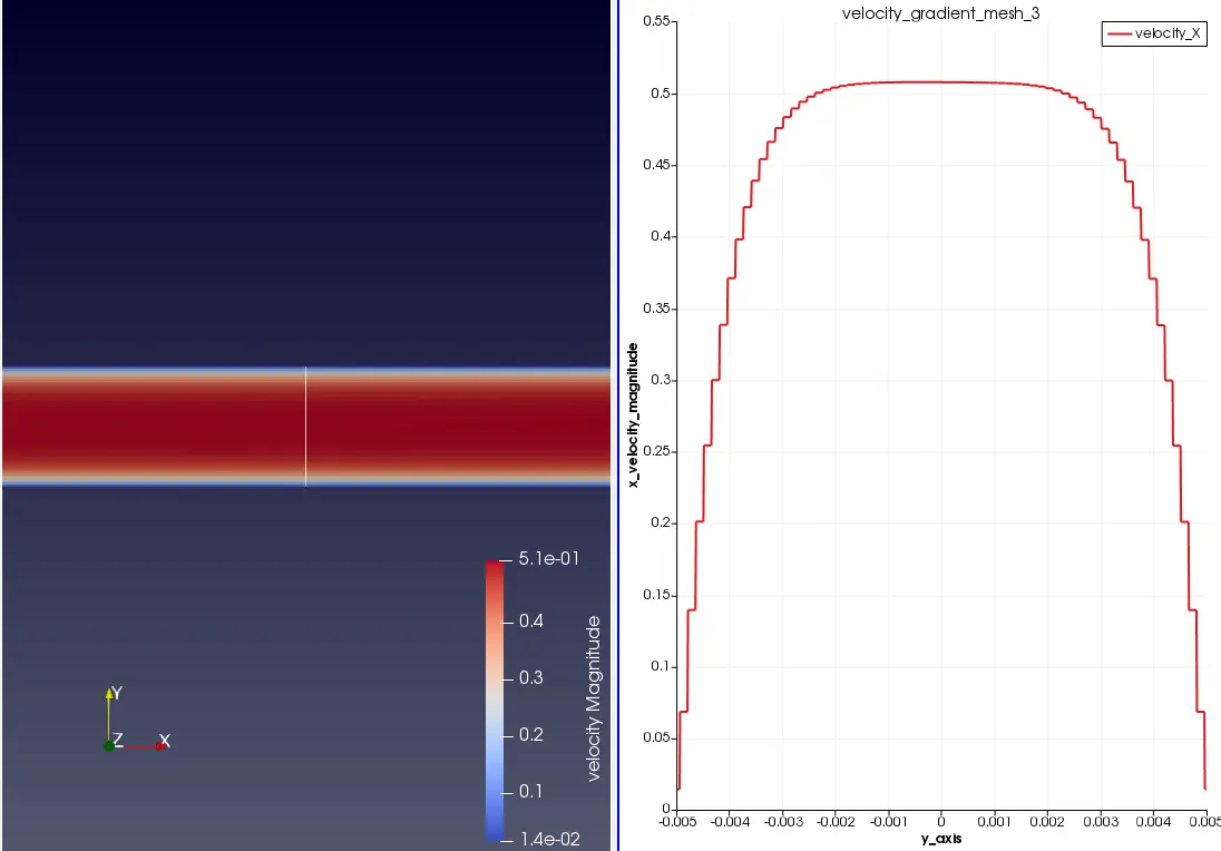
1. As expected the velocity profile across any cross section of the channel is parabolic because we have used wall boundary condition at the top and bottom face of the wall. And wall basically communicate through viscosity and due to that the velocity at the wall will become zero and gradually increases as we go towards the center of the channel.
2. Second observation is that as we refine the mesh the refinement of the velocity also occer. The maximum velocity increases as we increases the mesh cell count.

3. We have initiated the value of air with oxygen =77% and nitrogen to be 23% but after convergence it came to the original value.

Density Animation

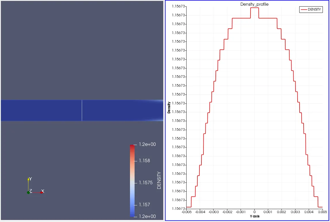
4. Density also follows the same profile pattern (parabolic) as velocity profile.

5 The solution converged around 48k cycle.

6. By seeing the pressure contour it is clear that the flow is drived by the pressure difference as we have said earlier.