Study of Buck converter using Control System Designer tool in matlab.
Questions:
1.
A] Explain the following terms and note down their mathematical formulae.
- Rise time
- Settling time
- Peak overshoot
- Steady state error
B] Tune a compensator for DC Motor Using Bode Diagram Graphical Tuning. The transfer function is given as-
`G=frac(1.5)(s^2+14s+40.20)`
Meet the following specifications - Rise time less than 0.5 seconds, Steady-state error of less than 5%, Overshoot of less than 10%, Gain margin greater than 20 dB, Phase margin greater than 40 degrees.
2.
Can a system with a pole on the right half of the s-plane be stable? Justify your answer with an example.
3.
Use the following link of Synchronous Buck Converter in order to solve the following questions:
A] Run the simulation for the default values and comment on the results with respect to stability of the system.
B] Change the reference voltage and comment on whether it is tracking the reference voltage or not.
C] Change the PI gain values and comment on the stability of the system w.r.t. new values.
D] Change the switching frequency and comment on the stability of the system w.r.t. new values.
Solution:
1.
A] Explain the following terms and note down their mathematical formulae.
- Rise time
- Settling time
- Peak overshoot
- Steady state error
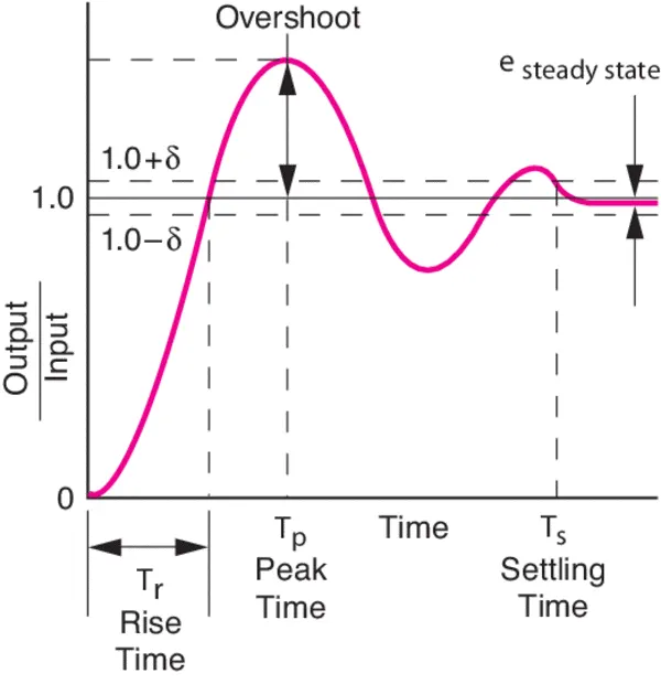
Fig01: Transient response parameters.
Rise time:
For applications in control theory, according to Levine (1996, p. 158), rise time is defined as "the time required for the response to rise from x% to y% of its final value", with 0% to 100% rise time common for underdamped second order systems, 5% to 95% for critically damped and 10% to 90% for overdamped ones. According to Orwiler (1969, p. 22), the term "rise time" applies to either positive or negative step response, even if a displayed negative excursion is popularly termed fall time.
t1 is the time at which the output of the system under analysis is at the x% of the steady-state value, while t2 the one at which it is at the y%, both measured in seconds.
tr is the rise time of the analysed system, measured in seconds. By definition,

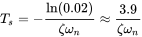
Settling time:
In control theory the settling time of a dynamical system such as an amplifier or other output device is the time elapsed from the application of an ideal instantaneous step input to the time at which the amplifier output has entered and remained within a specified error band.
Settling time includes a propagation delay, plus the time required for the output to slew to the vicinity of the final value, recover from the overload condition associated with slew, and finally settle to within the specified error.
Settling time is the time required for an output to reach and remain within a given error band following some input stimulus.
A general form is

Thus, if the damping ratio  , settling time to within 2% = 0.02 is:
Peak overshoot:
Peak overshoot Mp is defined as the deviation of the response at peak time from the final value of response. It is also called the maximum overshoot.
Mathematically, we can write it as
`Mp=c(tp)-c(infty )`
Where,
c(tp) is the peak value of the response.
c(∞) is the final (steady state) value of the response.
Steady state error:
The term steady-state error is used for the error that occurs between the set input to a control system and its output after it has settled down to its steady value. The steady-state error is a measure of the accuracy a control system has in tracking a command input.
A steady-state error is defined as the difference between the desired value and the actual value of a system when the response has reached the steady state.
Steady State errors for Unity Feedback Systems:
Consider the following block diagram of closed loop control system, which is having unity negative feedback.
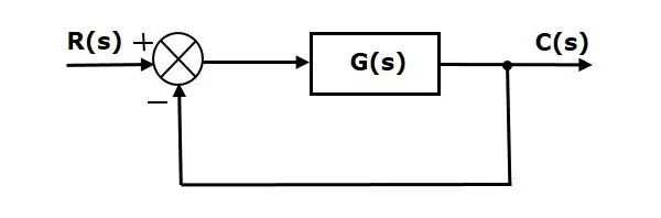
Where,
- R(s) is the Laplace transform of the reference Input signal r(t).
- C(s) is the Laplace transform of the output signal c(t).
We know the transfer function of the unity negative feedback closed loop control system as
`frac(C(s))(R(s))=frac(G(s))(1+G(s)`
`C(s)=frac(R(s)G(s))(1+G(s)`
The output of the summing point is -
`E(s)=R(s)-C(s)`
Substitute C(s) value in the above equation.
`E(s)=R(s)-frac(R(s)G(s))(1+G(s))`
`E(s)=frac(R(s)+R(s)G(s)-R(s)G(s))(1+G(s))`
`E(s)=frac(R(s))(1+G(s)`
Substitute E(s) value in the steady state error formula
`ess=lim_(s->0)frac(sR(s))(1+G(s))`
B] Tune a compensator for DC Motor Using Bode Diagram Graphical Tuning. The transfer function is given as-
`G=frac(1.5)(s^2+14s+40.20)`
Meet the following specifications - Rise time less than 0.5 seconds, Steady-state error of less than 5%, Overshoot of less than 10%, Gain margin greater than 20 dB, Phase margin greater than 40 degrees.
Following steps were involved in modifying the compensator:
- First the compensator was set according to the requirements of the overshoot and rise time.
- Then to satisfy the condition of steady state error integrator was added.
- The the values for phase margin and gain margin are checked.
- Further the pole (-25) and zero (-5) were added into the compensator.
- Finally the value of the compensator is edited (within 100) as per requirements of the step response by trial and error method.
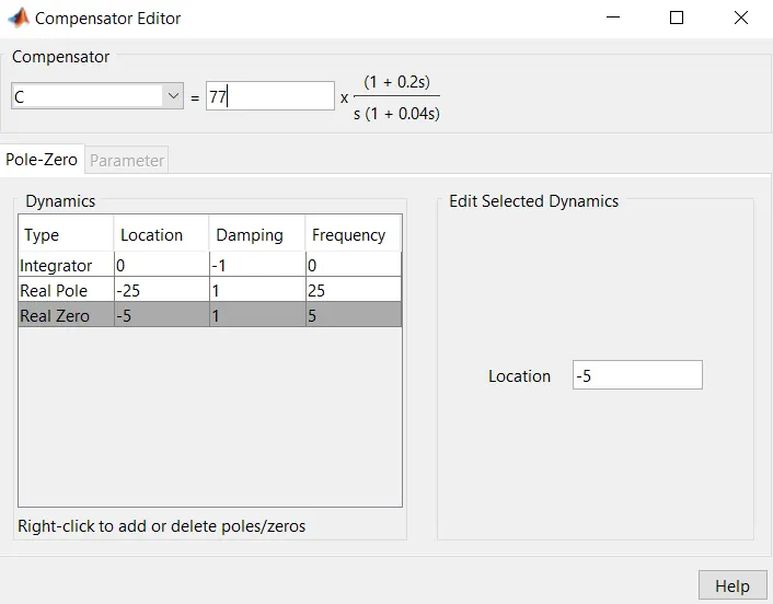
Fig02: Adding zeros and poles in compensator editor.
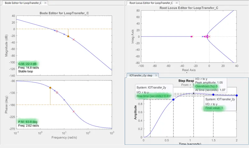
Fig03: Step response as per requirements for which the compensator is edited.
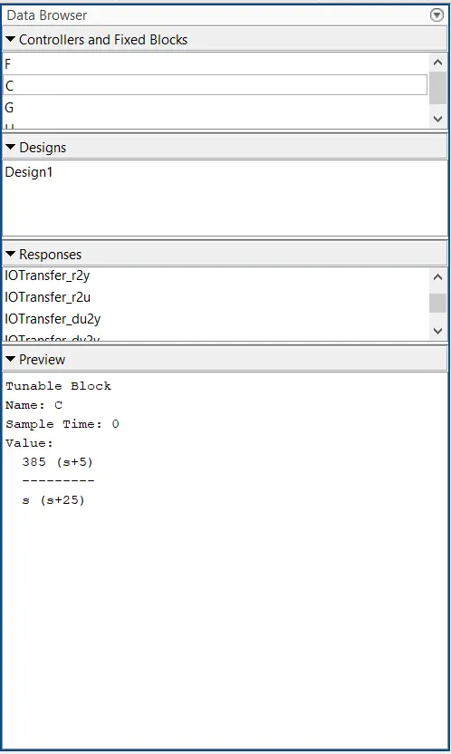
Fig04: Final value of the compensator as per the requirements of the step response.
2.
Can a system with a pole on the right half of the s-plane be stable? Justify your answer with an example.
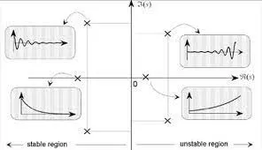
Fig05: For Linear Time Invarient (LTI) system if the input is bounded, the output must be bounded too.
Taking example:
- `G(s)=frac(s)((s+2)(s+3))`
- `H(s)=frac(s)((s+2)(s-1))`
For G(s) poles are:
s=-2 and s=-3
Laplace(G(s))=G(t)
`G(t)=K1.e^(-2t)+K2.e^(-3t)`
In this example both terms are decaying terms. Since both the terms are decaying, that means the output is bounded and hence the system is stable.
For the system to be stable both poles must lie on the LHS of the s-plane.
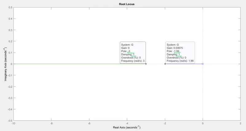
Fig06: Root locus plot for transfer function G.
Root locus gives us the value of the damping coefficient for the poles.
Here for s=-3 the damping coefficient is 1.
And for s=-2 the damping coefficient is 1.
A positive damping coefficient means continuous decrease in amplitude. Which means a bounded output and hence a stable system.
For H(s) poles are:
s=-2 and s=1
Laplace(H(s))=H(t)
`H(t)=K1.e^(-2t)+K2.e^(t)`
The first term is decaying term while the second term is rising term. This is the benefit of applying laplace's transformation it allows us to check whether the output is bounded or not.
Since the second terrm is rising indefinitely, that means the output is not bounded and hence the system is unstable. For the system to be stable both poles should be on the LHS of the s-plane.
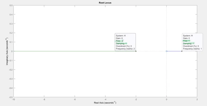
Fig07: Root locus plot for transfer function H.
Root locus gives us the value of the damping coefficient for the poles.
Here for s=-2 the damping coefficient is 1.
And for s=1 the damping coefficient is -1.
A negative damping coefficient means continuous increase in amplitude. Which means a unbounded output and hence a unstable system.
3.
Use the following link of Synchronous Buck Converter in order to solve the following questions:
A] Run the simulation for the default values and comment on the results with respect to stability of the system.
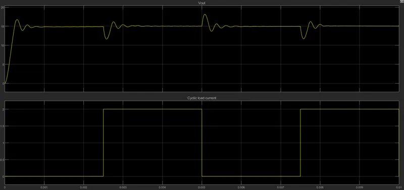
Fig08: Results for default values of the synchronous buck converter system.
This example shows the synchronous buck converter where the switched power supply converts a 30V DC supply into a regulated 15V DC supply.
Therefore default results shows the output maintained at 15V after each repeated cycle.
That means the output voltage is bounded and system is a stable system.
B] Change the reference voltage and comment on whether it is tracking the reference voltage or not.
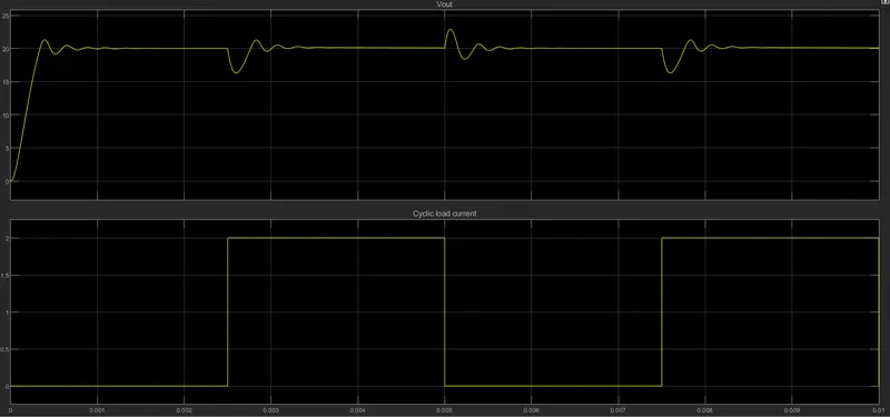
Fig09: Results for changed value of reference voltage (20V) of the synchronous buck converter system.
Here we changed the value of the reference voltage to 20V and simulate the model for the results.
As per reference value the output of the system is also regulated as 20V.
That means the output voltage is bounded and system is a stable system. Changing the reference value does not affect the stability of the system.
C] Change the PI gain values and comment on the stability of the system w.r.t. new values.
i] Ki=200 and Kp=0.5
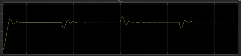
Fig10: Result for Ki=200 and Kp=0.5
ii] Ki=5 and Kp=10
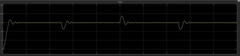
Fig11: Result for Ki=5 and Kp=10
iii] Ki=200 and Kp=0.01
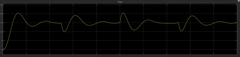
Fig12: Result for Ki=200 and Kp=0.01
Varying the integral gain (Ki) of the system affects the stability of the system and can make system unstable.
Varying the praportional gain (Kp) of the system affects the stability of the system and can make system unstable..
Thus both must be varied (increased or decreased) w. r. t. one another so that the stability of the system is maimtained.
D] Change the switching frequency and comment on the stability of the system w.r.t. new values.
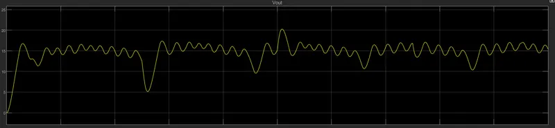
Fig13: Result for frequency of 500Hz.
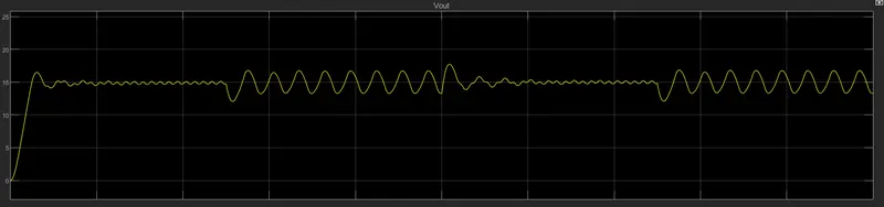
Fig14: Result for frequency of 10000Hz.
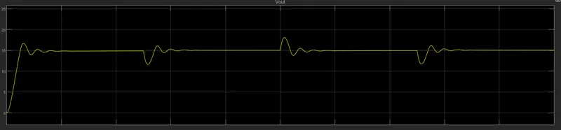
Fig15: Result for frequency of 150000Hz.
Greater the switching frquency greater is the stability of the system.
Lower switching frequency results in unstable system.