Flow over bicycle

AIM- Python code for Drag force against a cyclist

GOVERNING EQUATION-

Drag Force = 0.5* (density)* (area)* (velocity)^2

BODY-

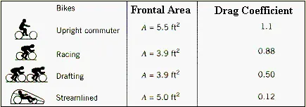
A cyclist changes his/her frontal area to adjust the drag according to the situation. In this project we have considered only racing posture. Drafting posture is when cyclist move behind each other to take advantage of the wake as drag is reduced. Futher explanation has been shown in the figure below. The pattern in decrease in drag coefficient can be see with decrease in frontal area. However, in the streamlined position, the drag coefficient reduces because of the flow over the body and shifting of seperation point more in the downstream of the flow.

The code is explained as follows –

The importing for libraries like matplotlib.pyplot (for matlab functions) and numpy( for mathematical operation over arrays) is done by the first three codes

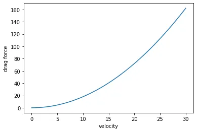
In case I, the various variables are used which are of density(rho), frontal area(A),drag coefficient(C) and velocity(V). Here, the changing velocity for a cyclist during transition from racing posture is taken into consideration in the range of [0m/s to 30m/s].linspace command from the numpy library is used to give linear spaced velocity .The frontal area remains constant of 0.334m^2. The co-efficient of drag for the cyclist ia to be taken as 0.88. The drag force is calculated by a for loop. The range is defined for the length of velocities and then drag force value is appended and saved into a void defined earlier as “drag_force = []”. The print command is to display the result at the end of the loop. The plot command which is called from the matplotlib library is used to generate the graph with defined x axis and y axis with commands 'plt.xlabel' and 'plt.ylabel'

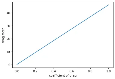
In the case II, the various variables are used which are of density(rho), frontal area(A),drag coefficient(C) and velocity(V). Here, the drag coefficent for a cyclist during transition from racing posture to drafting posture is taken into consideration in the range (0.5 to 0.88). Drafting is the arrangement in which cyclist go in a straight path to reduce drag. Again, linspace command from numpy library is used to give linear spaced Cd values. The frontal area remains constant. the velocity of the cyclist is to be taken as 15 m/s. The drag force is calculated by a for loop. The range is defined for the length of velocities and then drag force value is appended and saved into a void defined earlier as “drag_force = []”. The print command is to display the result at the end of the loop. The line command used to generate the graph with defined x axis and y axis with commands 'xlabel' and 'ylabel'.

import matplotlib.pyplot as plt #library for matlab plots
import numpy as np              #library for mathematical operations over arrays


#frontal area
A= 0.334

#density
rho = 1.225

#CASE 1

#velocity of cyclist
v_1 = np.linspace(0,30,60)

#coefficient of drag
cd = 0.88


#drag force
drag_force1 = []  #to store the value of drag forces
for V in v_1 :
    drag_force1.append( 0.5*rho*A*cd*(pow(V,2))) #to calculate the drag force

print(drag_force1)         #to show result
plt.plot(v_1,drag_force1)  #to plot graph
plt.xlabel('velocity')
plt.ylabel('drag force')
plt.show()                 #to show the plotted graph

#CASE 2

#velocity of cyclist
v_2 = 15
#coefficient of drag
cd_2 = np.linspace(0,1,10)

#drag force
drag_force2 = []
for cd in cd_2 :
    drag_force2.append( 0.5*rho*A*cd*(pow(v_2,2)))

print(drag_force2)
plt.plot(cd_2,drag_force2)  #to plot graph
plt.xlabel('coefficient of drag')
plt.ylabel('drag force')
plt.show()

CONCLUSION-

• The drag force follows parabolic curve because of quadratic function of velocity. At lower velocity, the drag force is comparitively less where as a spike in drag force is seen as the velocity increases. The slope of the curve continuous increases.
• 
• The drag force follows linear curve because of linear function of drag coefficient. At lower drag coefficient, the drag force is comparitively less and a linear increase in drag force is seen as the drag coefficent increases. The slope of the curve remains constant.
•