Steady Vs Unsteady flow over a cylinder

Aim:- The aim of this challenge is to Simulate the flow over a cylinder and explain the phenomenon of Karman vortex street.

Introduction:-There are two parts given for which the simulation has been asked.

PART-I

1. Here it has been asked to simulate the flow with the steady and unsteady case and calculate the Strouhal Number for Re= 100.

PART-II

1. Here it is needed to calculate the coefficient of drag and lift over a cylinder by setting the Reynolds number to 10,100,1000,10000 & 100000. (Run with steady solver)
2. And discuss the effect of Reynolds number on the coefficient of drag. [ Results should be validated with any standard literature and error should be within 5 %]

Solving & Modelling Approach:-

The paper presents the simulation of a flow over a 2D cylinder with inflow velocity 1m/s and the outlet is atmospheric pressure by creating a customise fluid and modifying the Reynolds Number. Also vortex shedding is visualised with addition of a moniter point for measuring any parameter such as pressure,velocity etc. The paper also presents animation files, numerical diffusion, steady vs transient analysis and post processing.

Pre-processing and solver setting:-

At first we drag the Fluid Flow Fluent solver from the toolbox to the Project Schematic View and start with the geometry. In the geometry the computational domain is rectangular which is basically 2D and within it a slice of a cylinder is drawn. The diameter(D) of the cylinder is 2m and the distance towards the left and right of the cylider where the boundaries of the domain are drawn is 10D (left from centre of cylinder) & 20D (right from centre of cylinder). Now the top and bottom boundaries(Symmetry) are 5D each from the centre of the cylinder. The total length is 60 m and width is 20m. The following figures shows the pre processing and solver setting before going into the process for the problem in part 1.

(a) The analysis is first done of steady

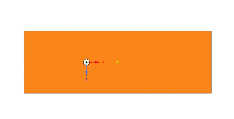
Fig 1 Computational Domain

The above figure is the surface of the computational domain upto which is the interest lies.

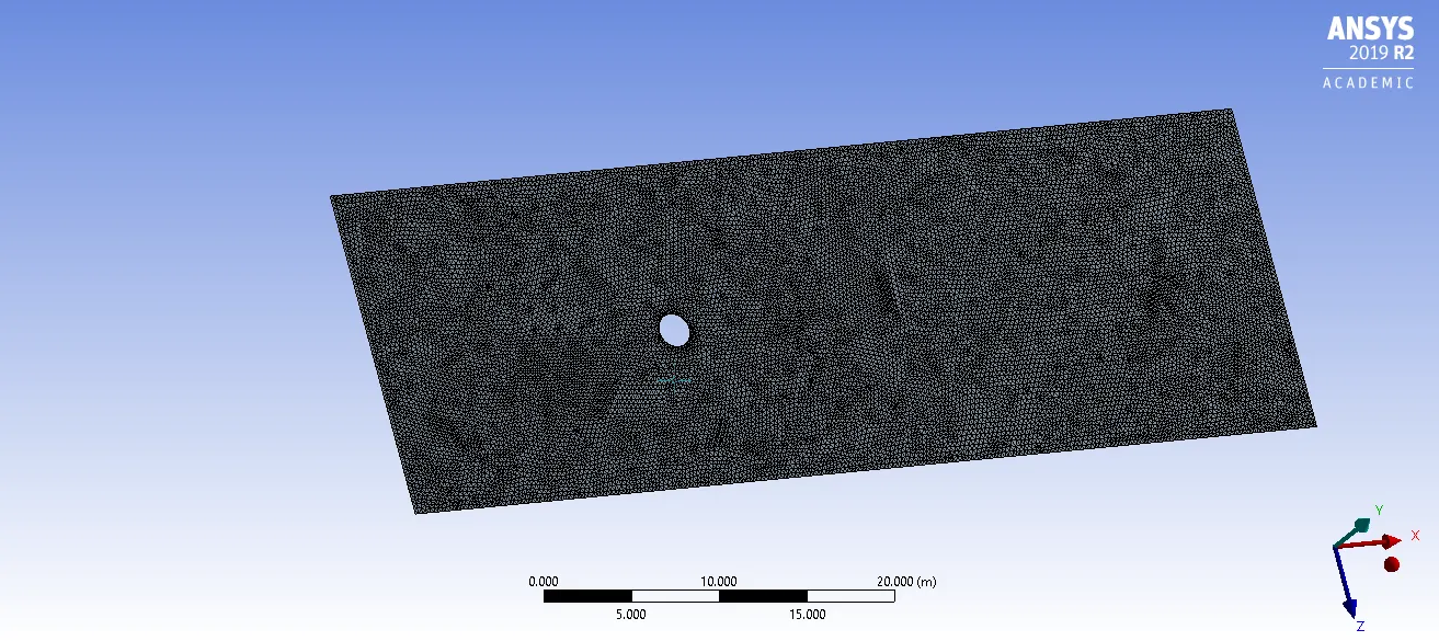
Fig 2 Meshing with element size 0.25m

Figure no 2 shows the mesh generated in the domain. The default mesh was quadrilateral but to make the analysis more refine triangular mesh with elememt size 0.25m is used. Also the name of the sides are also created as left side is inlet, right as outlet, and top-bottom are symmetry & cylinder wall.

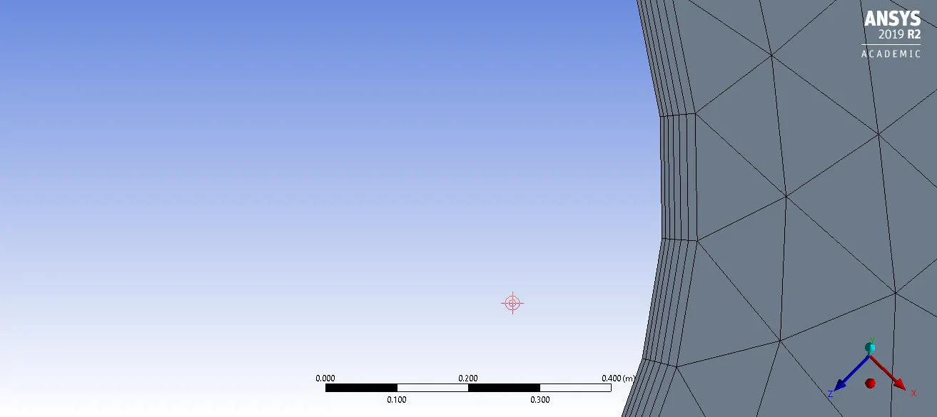
Fig 3 Selecting 6 inflation layers

Since the flow around the cylinder is more important so inflation layers are also included. This helps in creating body fitted mesh as it completely fits the mesh where the first layer thickness is 0.005m with growth rate of 20%.

After this in the solution section the required solver settings are made- steady state, pressure based, velocity is absolute, laminar flow, material is air with dynamic viscosity of 0.020, density is 1, inlet velocity 1 m/s, outlet pressure 1atm, for cylinder wall no slip BC is used. Now a moniter point is also created at the centre of the domain so to find the parameters across it. To know the different flow quantities a surface report on vertex average of velocity and pressure is created on the moniter point.

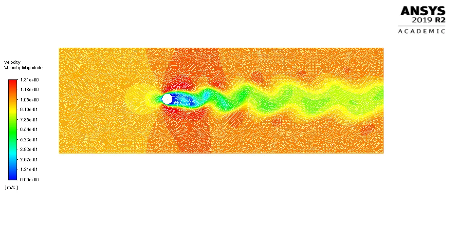
Fig 4 Velocity Contour showing Vortex Shedding

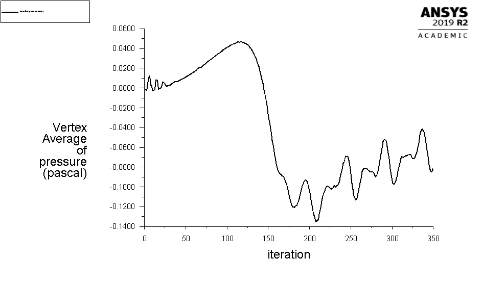
Fig 5 Vertex Average of Pressure

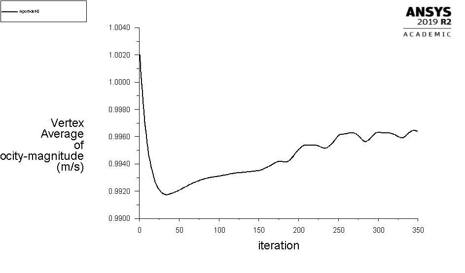
Fig 6 Vertex Average of Velocity

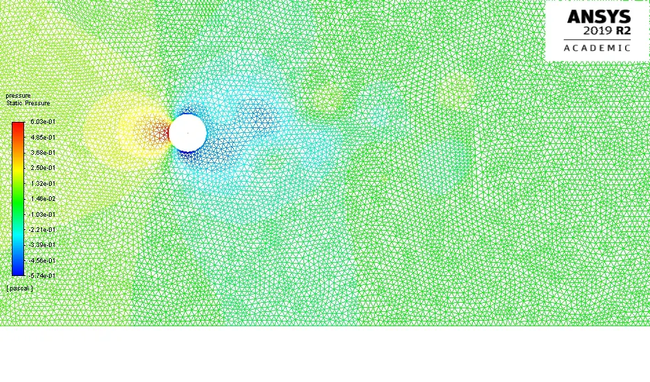
Fig 7 Pressure Contour

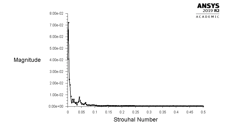
Fig 7 Strouhal Number based on the moniter point

(b) The analysis is done for unsteady flow with Re=100.

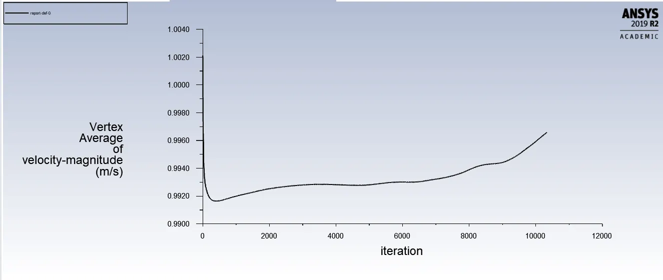
Fig 8 Vertex Average of Velocity

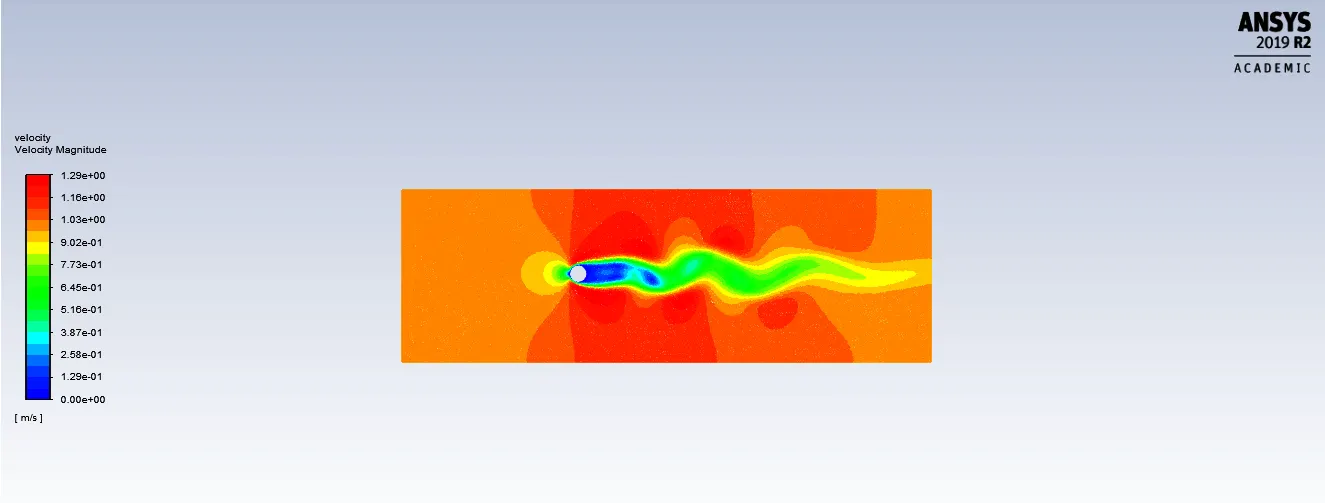
Fig 9 Velocity Contour showing Vortex Shedding

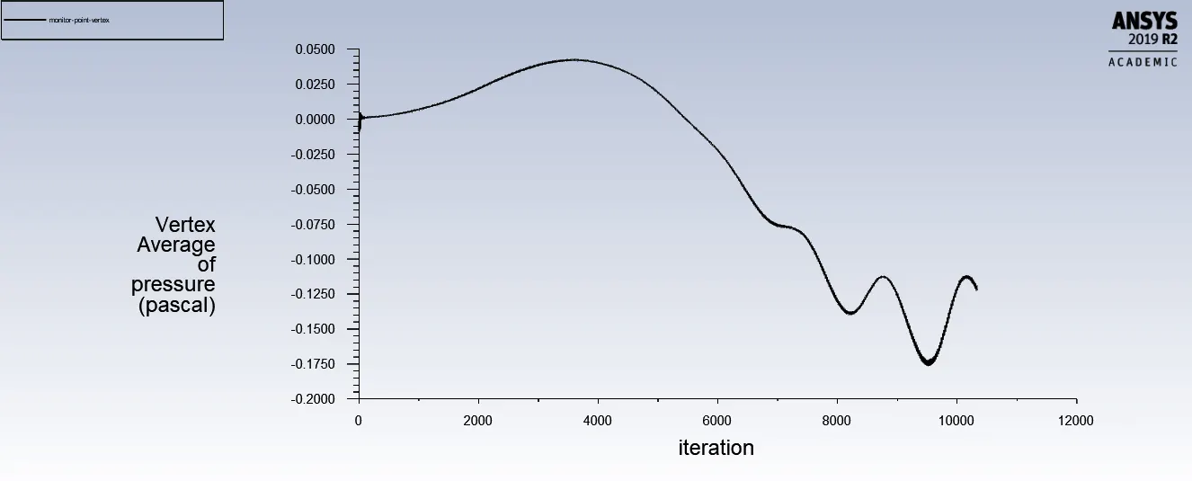
Fig 10 Vertex Average of Pressure

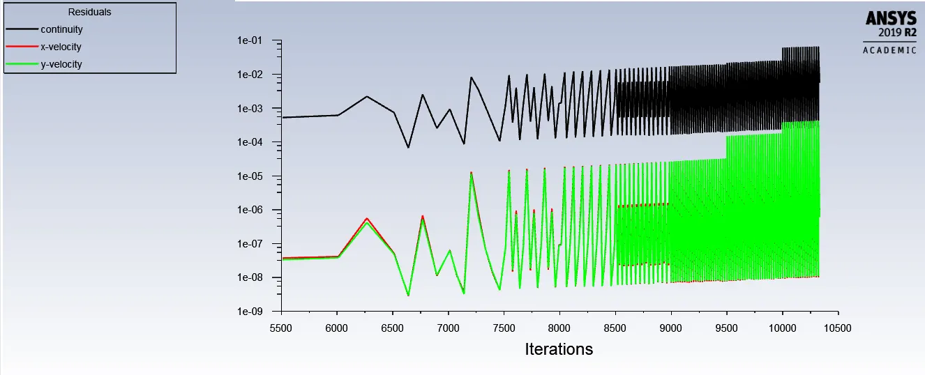
Fig 11 Residuals

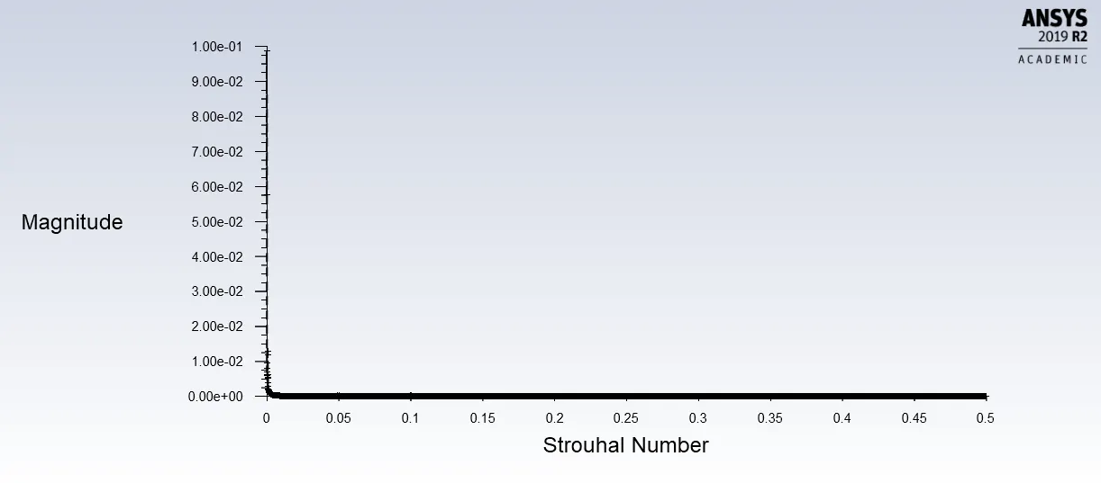
Fig 12 Strouhal Number based on the moniter point

PART-II Reynolds number to 10

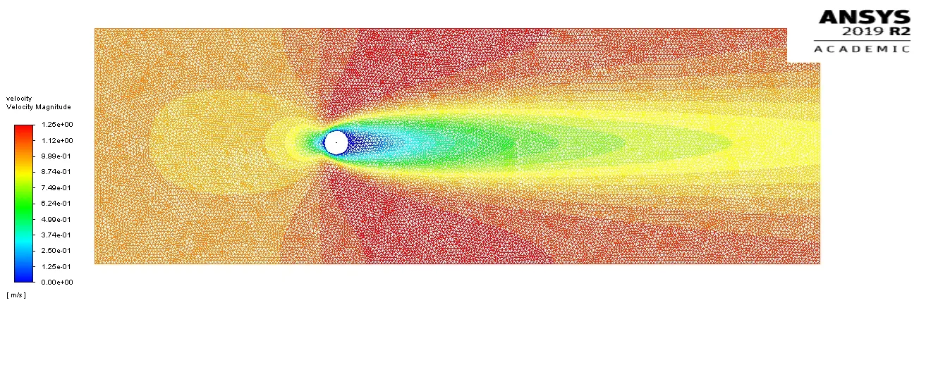
Fig 13 Velocity Contour showing Vortex Shedding

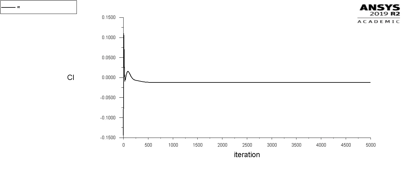
Fig 14 Co efficient of lift based on the moniter point

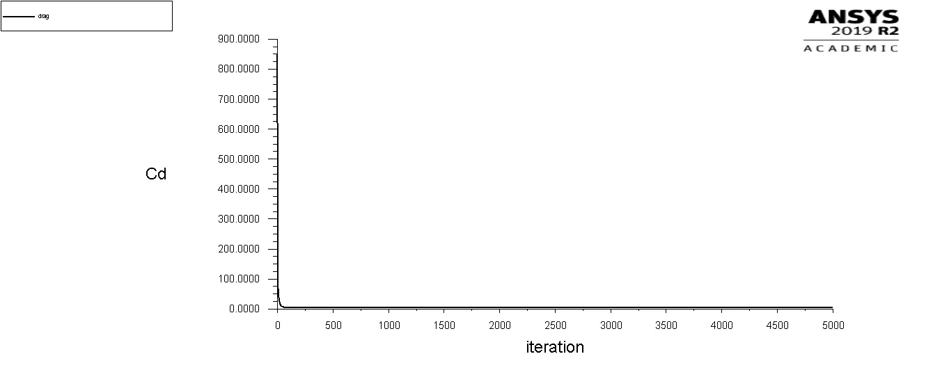
Fig 15 Co efficient of drag based on the moniter point

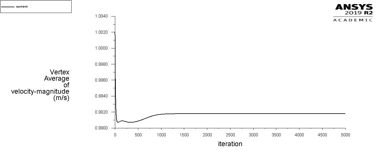
Fig 16 Vertex Average of Velocity

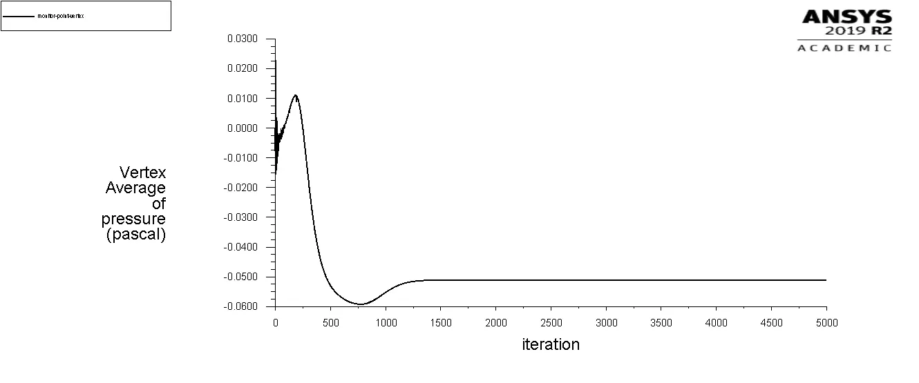
Fig 17 Vertex Average of Pressure

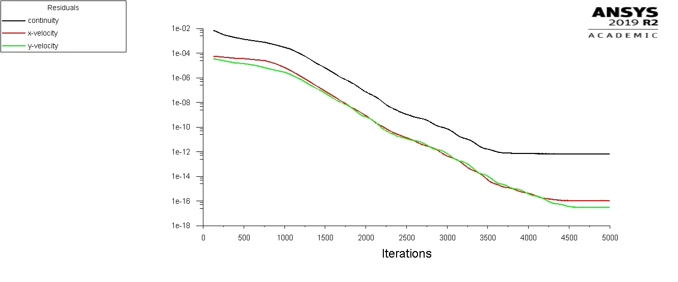
Fig 18 Residuals

Reynolds number to 100

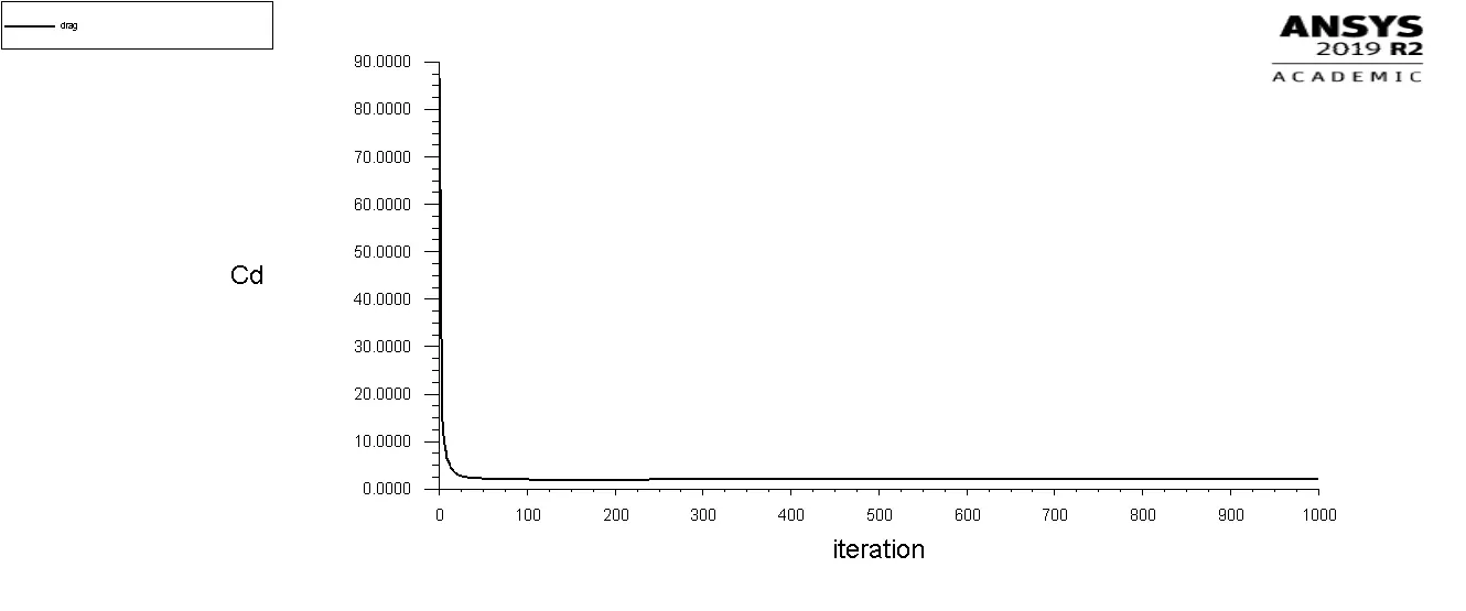
Fig 19 Co efficient of drag based on the moniter point

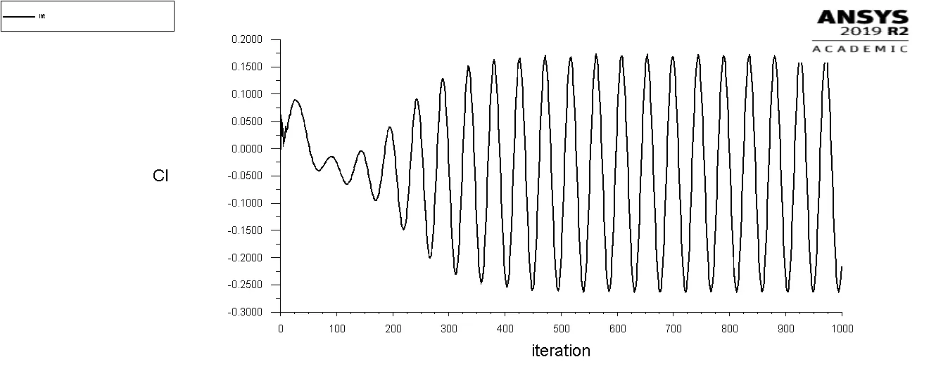
Fig 20 Co efficient of lift based on the moniter point

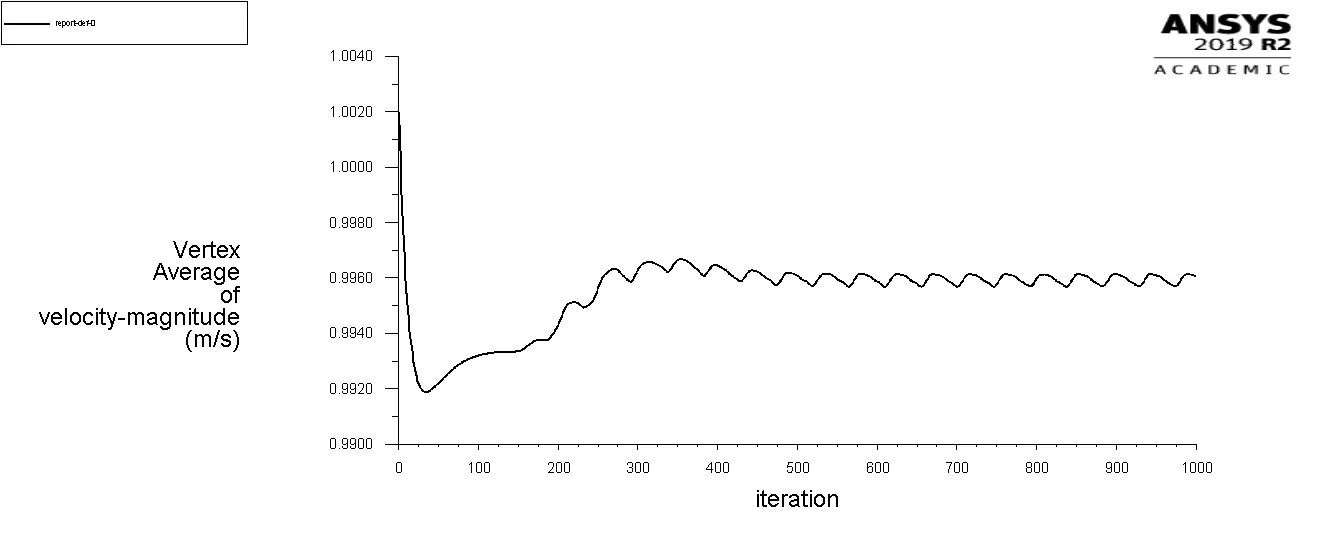
Fig 21 Vertex Average of Velocity

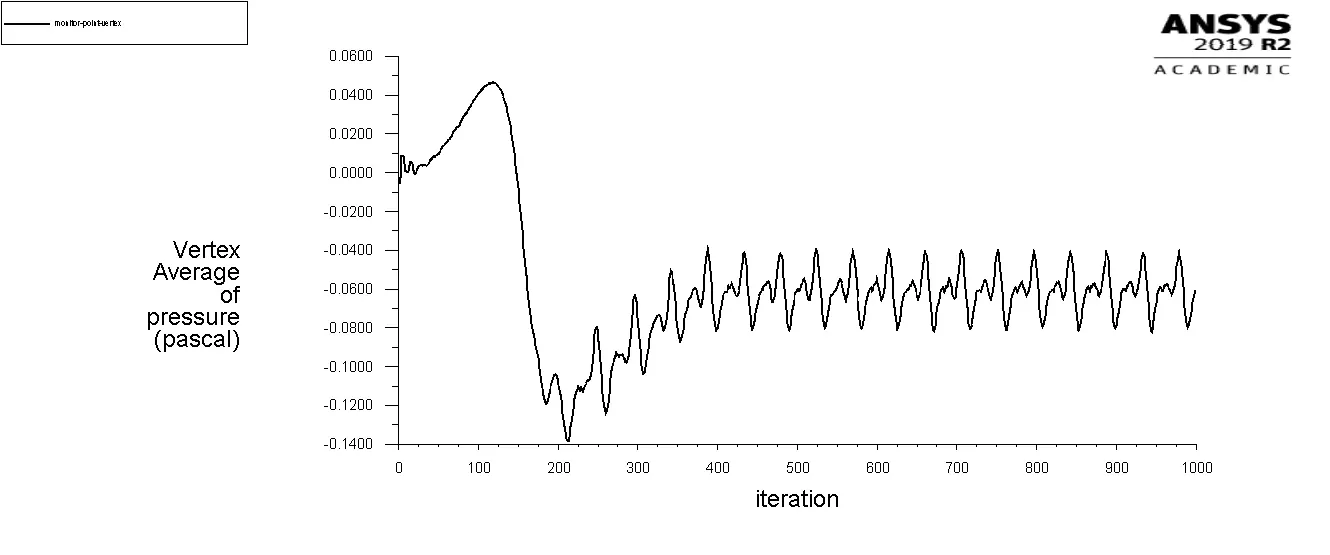
Fig 22 Vertex Average of Pressure

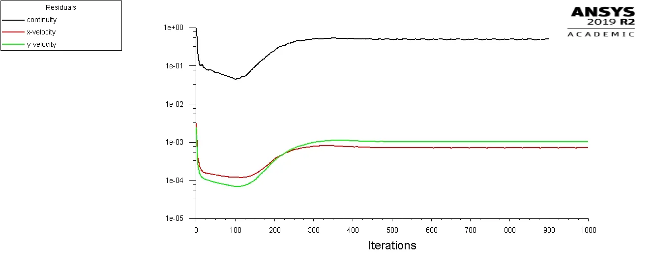
Fig 23 Residuals

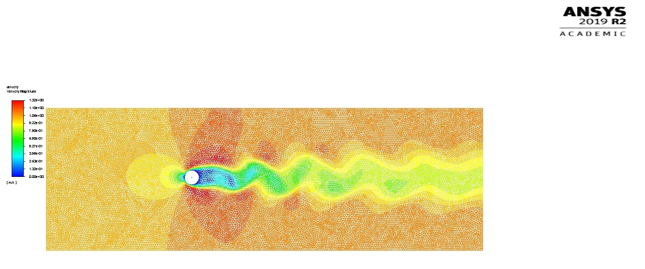
Fig 24 Velocity Contour showing Vortex Shedding

Reynolds number to 1000

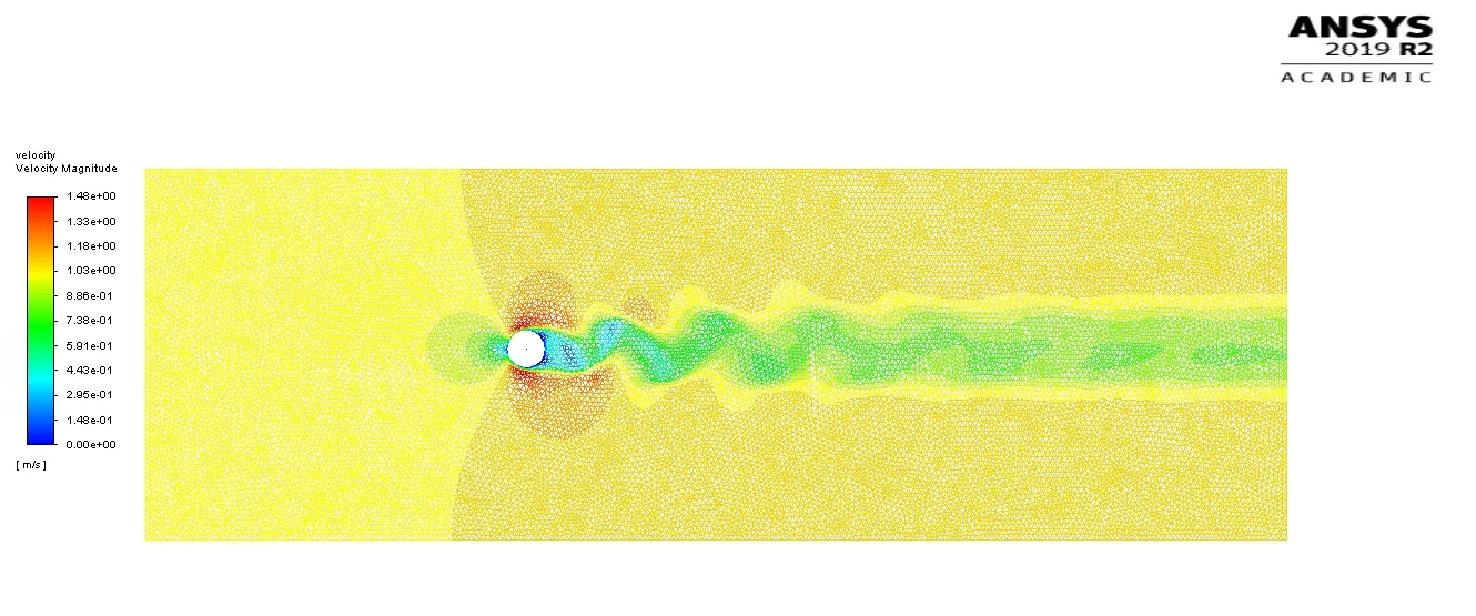
Fig 25 Velocity Contour showing Vortex Shedding

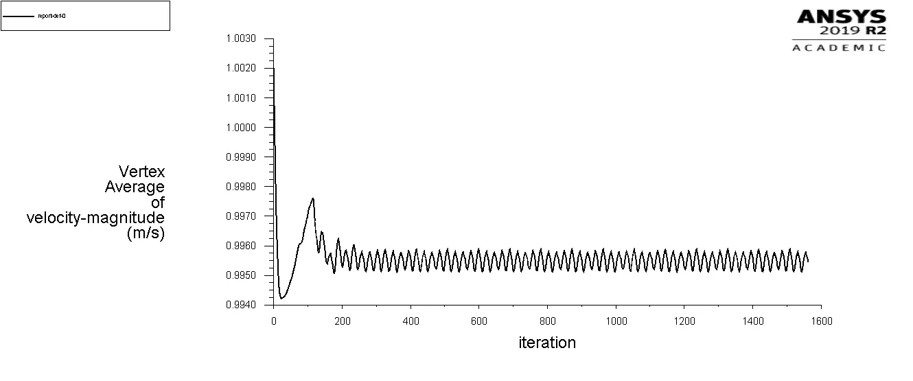
Fig 26 Vertex Average of Velocity

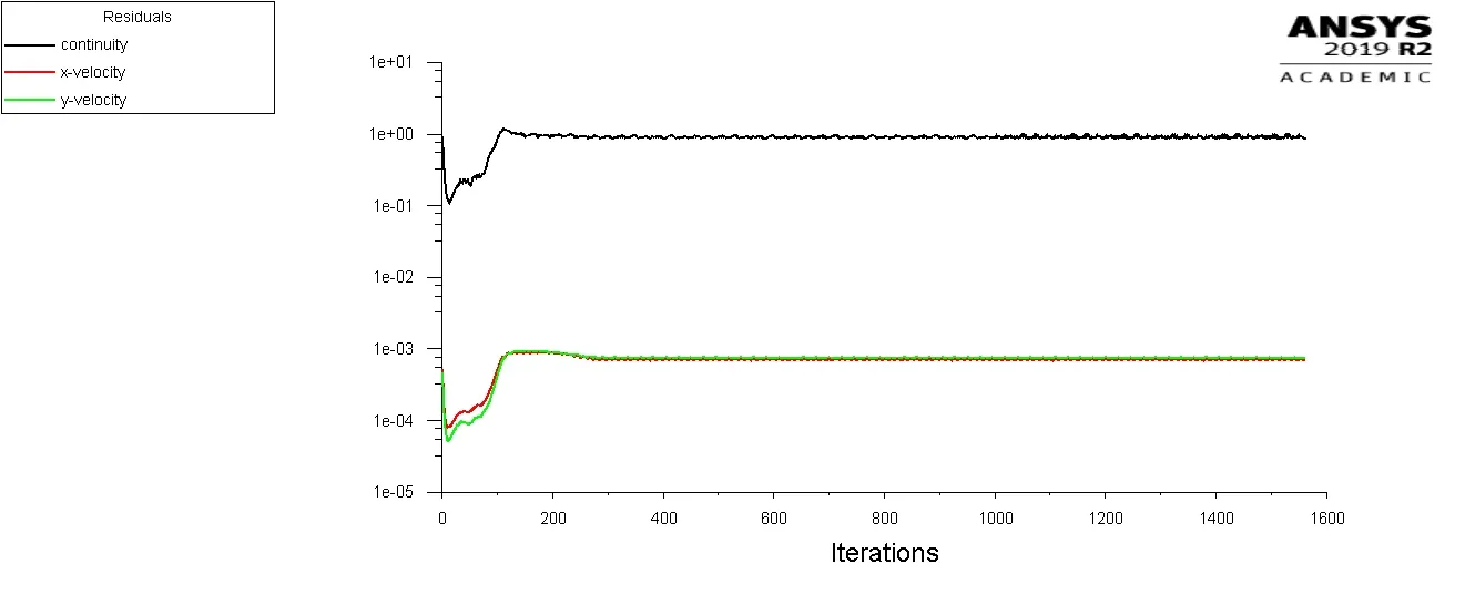
Fig 27 Residuals

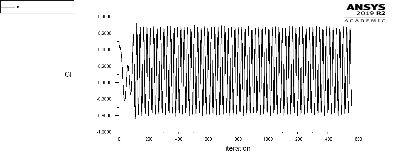
Fig 28 Co efficient of lift based on the moniter point

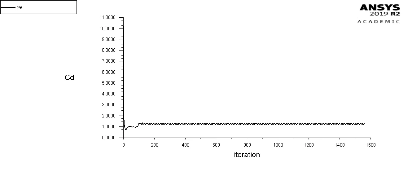
Fig 29 Co efficient of drag based on the moniter point

Reynolds number to 10000

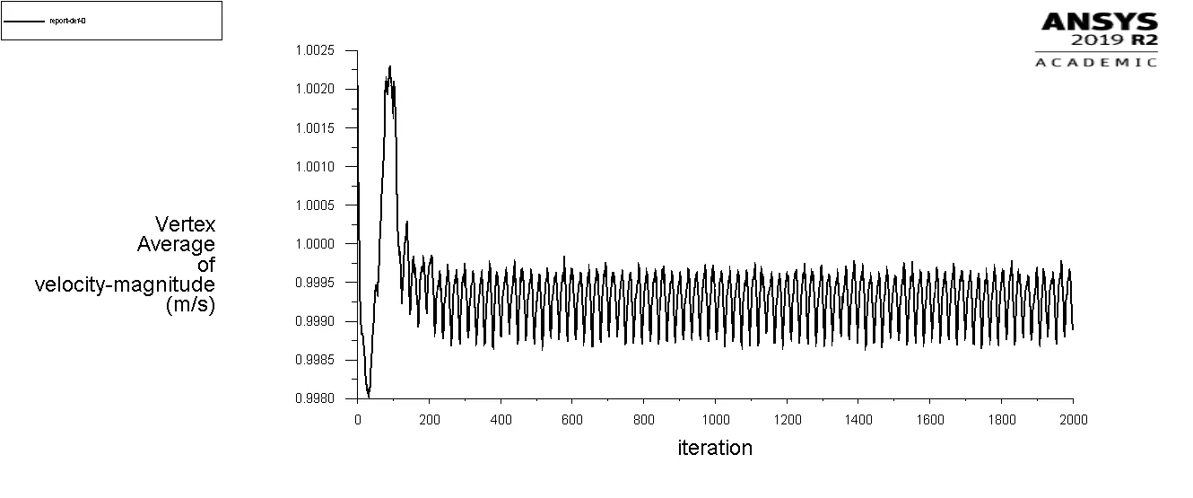
Fig 30 Vertex Average of Velocity

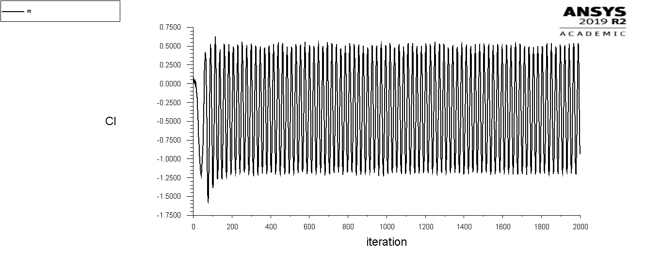
Fig 31 Co efficient of lift based on the moniter point

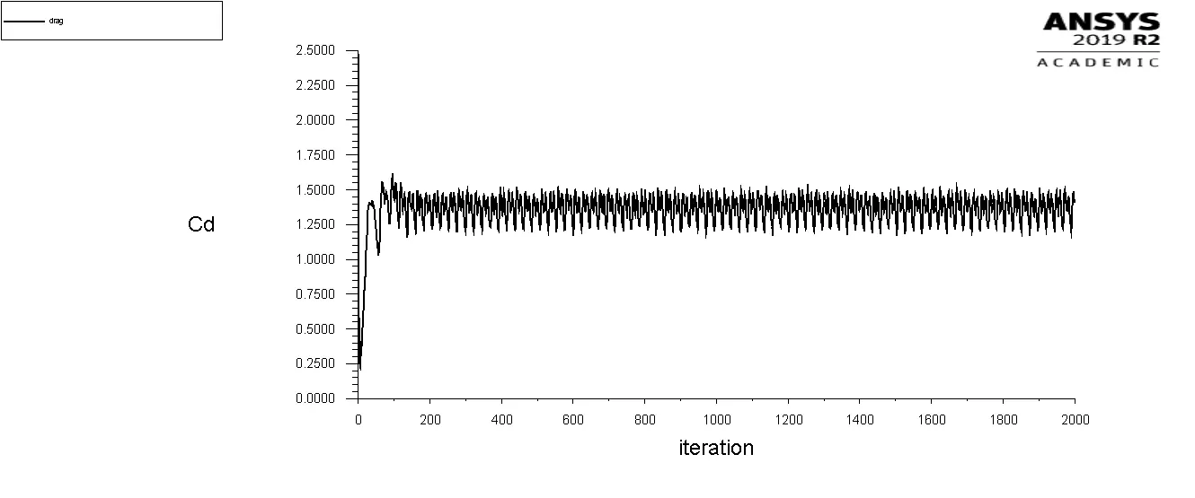
Fig 32 Co efficient of drag based on the moniter point

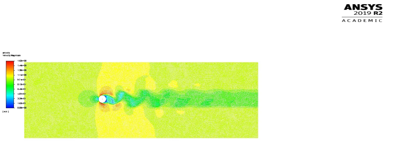
Fig 33 Velocity Contour showing Vortex Shedding

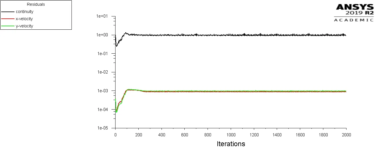
Fig 34 Residuals

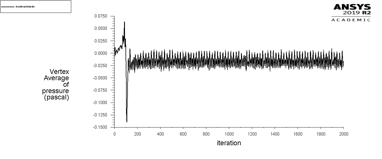
Fig 35 Vertex Average of Pressure

Reynolds number to 100000

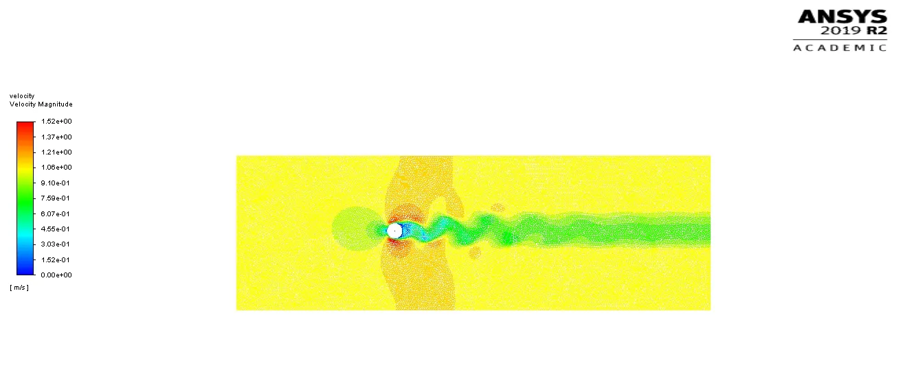
Fig 36 Velocity Contour showing Vortex Shedding

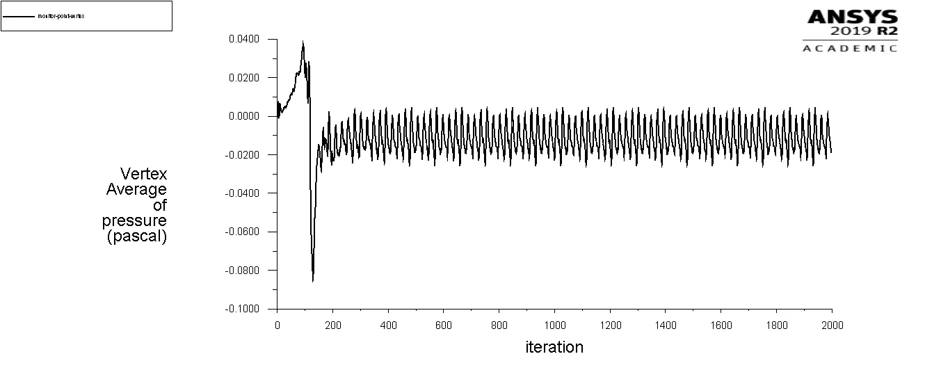
Fig 37 Vertex Average of Pressure

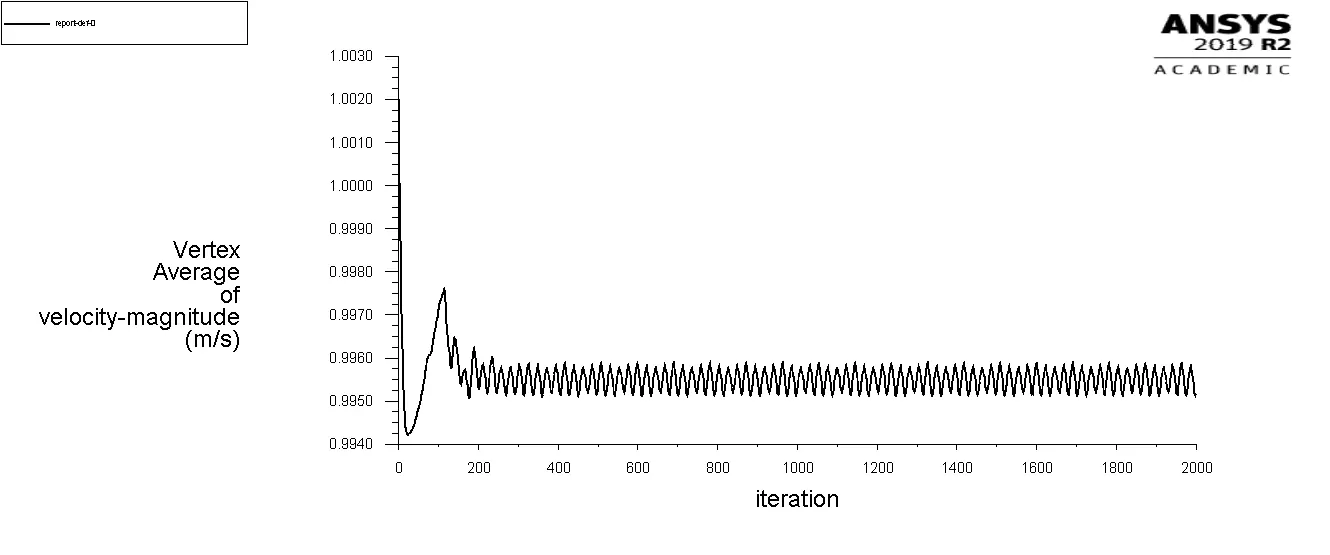
Fig 38 Vertex Average of Velocity

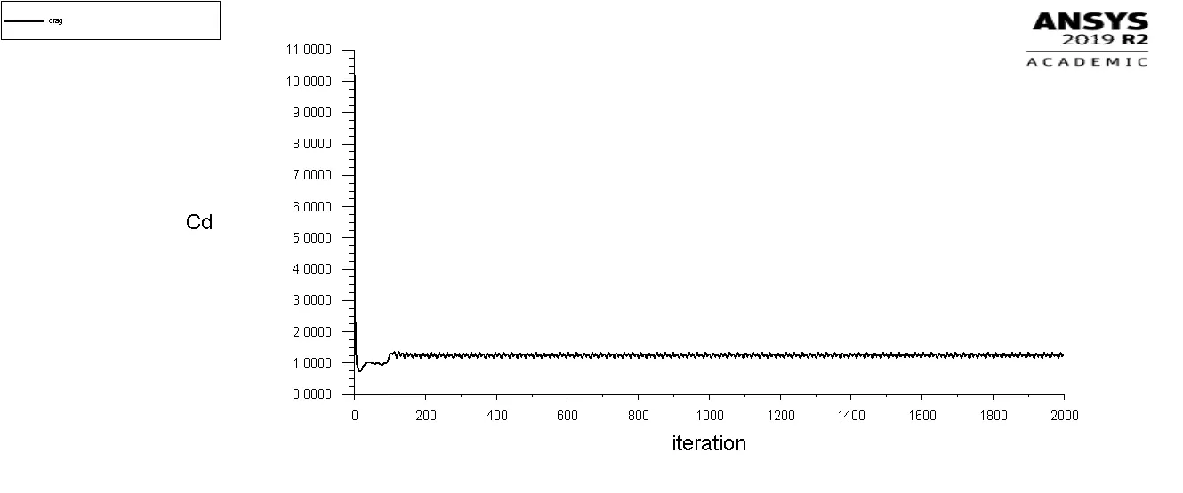
Fig 39 Co efficient of drag based on the moniter point

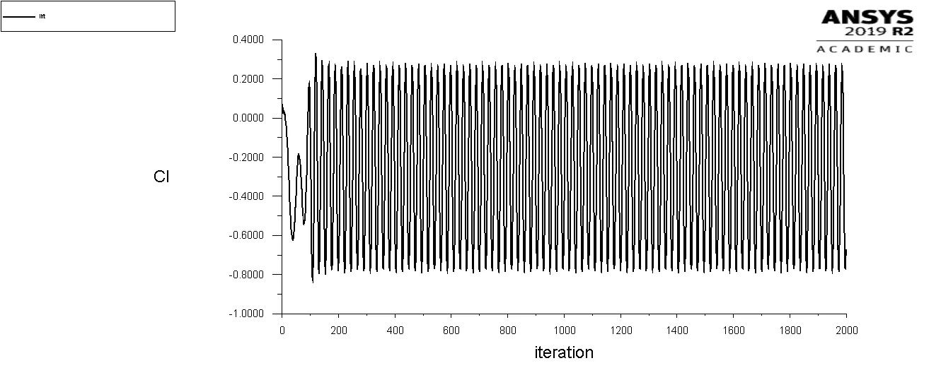
Fig 40 Co efficient of lift based on the moniter point

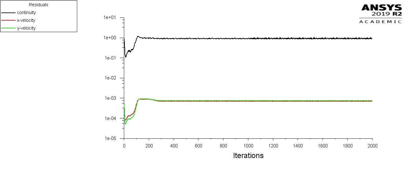
Fig 41 Residuals

Conclusion:- With change in Reynolds Number the fluctuation rises, for low Re there is less fluctuation and for more Re there is more fluctuation