Flow over a cylinder
AIM
The main aim of this project is to simulate the flow over the cylinder
OBJECTIVES
The main objectives of the simulation are
- simulate the karman vortex street concept
- running the simulation for steady and transient case of flow
- calculate the lift and drag coefficient
KARMAN VORTEX STREET
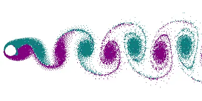
In fluid dynamics, vortex shedding is an oscillating flow that takes place when a fluid such as air or water flows past a bluff body at certain velocities, depending on the size and shape of the body. In this flow, vortices are created at the back of the body and detach periodically from either side of the body forming a Von Karmaan vortex street. The fluid flow past the object creates alternating low-pressure vortices on the downstream side of the object. The object will tend to move toward the low-pressure zone. If the bluff structure is not mounted rigidly and the frequency of vortex shedding matches the resonance frequency of the structure, then the structure can begin to resonate, vibrating with harmonic oscillations driven by the energy of the flow.
Kármán vortex street is a repeating pattern of swirling vortices, caused by a process known as vortex shedding, which is responsible for the unsteady seperation of flow of a fluid around blunt bodies. For common flows (the ones which can usually be considered as incompressible or isothermal), the kinematic viscosity is everywhere uniform over all the flow field and constant in time, so there is no choice on the viscosity parameter, which becomes naturally the kinematic viscosity of the fluid being considered at the temperature being considered. On the other hand, the reference length is always an arbitrary parameter, so particular attention should be put when comparing flows around different obstacles or in channels of different shapes: the global Reynolds numbers should be referred to the same reference length. This is actually the reason for which most precise sources for airfoil and channel flow data specify the reference length at a pedix to the Reynolds number. The reference length can vary depending on the analysis to be performed: for a body with circle sections such as circular cylinders or spheres, one usually chooses the diameter; for an airfoil, a generic non-circular cylinder or a bluff body or a revolution body like a fuselage or a submarine, it is usually the profile chord or the profile thickness, or some other given widths that are in fact stable design inputs; for flow channels usually the hydraulic diameter about which the fluid is flowing.
FLOW OVER CYLINDER FOR STEADY STATE
The general stages involved for the flow over the cylinder are
- Geometry
- Mesh
- Setup
- Solution
Geomerty
The first step in the geometry is to create a sketch in the XZ plane according to the dimensions and then exit to the isometric view. For the sketch first we create the circle and then draw an 60x20 metre dimensional plane and draw a sketch of 2m. Then we select the pull tool to create the surface and then save the geometry file.
Mesh
During the mesh generation process we create a triangular mesh with a mesh size of 0.25 m. When we process the sizing factor we create 36 number of divisions for the cylinder, sizing is defined as the number of divisions for an edge in the geometry. the number of elements for the mesh is 40502 elements during the mesh generation process. Now we are adding additional layers to the edge of the cylinder to capture the Karman vortex street. The process of adding extra layers to capture the physics of the flow accurately is known as inflation layers. For this case we are adding 6 layers of additional mesh layers.
Setup
In order to setup the korman vortex street effect for the flow over the cylinder we have to follow these steps
- Solver - pressure based solver
- Solver state - steady state simulation
- Model - laminar flow model
- Fluid used - user defined (air)
- boundary conditions -
- Inlet velocity - 1m/s
- density of air - 1 kg/m^3
- viscosity - 0.02 kg-m/s
In the steady state solution we see that the simulation has run for 500 iterations and we see the solution converges after 400 iterations. The residual plot shows continuity, x-velocity, y-velocity parameters for which we are running the simulation.
In this simulation we create a monitor point at a distance of 4 times diameter, which is used to monitor the velocity of the vortex average of the velocity. after 200 iterations we see the formation of the waves and as we move through the simulation the formation of vortex street is formed.
RESULTS
Velocity contour plot
The velocity contour plot is shown in the above image as the flow develops we observe the karman vortex street effect in the steady state simulations and we see the velocity distribution across the domain of the simulation. Initially we can see that the vortex is being generated at the wall of the cylinder and as we go along the length of the plane vortices are formed.
Pressure Contour
The static pressure variation is shown for this simulation and then the pressure distribution is shown where the gauge pressure is zero. Due to the vortex there is a pressure drop across the wall of the cylinder.
FLOW OVER CYLINDER FOR UNSTEADY STATE
The general stages involved for the flow over the cylinder are
- Geometry
- Mesh
- Setup
- Solution
Geomerty
The first step in the geometry is to create a sketch in the XZ plane according to the dimensions and then exit to the isometric view. For the sketch first we create the circle and then draw an 60x20 metre dimensional plane and draw a sketch of 2m. Then we select the pull tool to create the surface and then save the geometry file.
Mesh
During the mesh generation process we create a triangular mesh with a mesh size of 0.25 m. When we process the sizing factor we create 36 number of divisions for the cylinder, sizing is defined as the number of divisions for an edge in the geometry. the number of elements for the mesh is 40502 elements during the mesh generation process. Now we are adding additional layers to the edge of the cylinder to capture the Karman vortex street. The process of adding extra layers to capture the physics of the flow accurately is known as inflation layers. For this case we are adding 6 layers of additional mesh layers.
Setup
In order to setup the korman vortex street effect for the flow over the cylinder we have to follow these steps
- Solver - pressure based solver
- Solver state - unsteady state simulation
- Model - laminar flow model
- Fluid used - user defined (air)
- boundary conditions -
- Inlet velocity - 1m/s
- density of air - 1 kg/m^3
- viscosity - 0.02 kg-m/s
In the unsteady state solution we see that the simulation has run for 500 iterations and we see the solution converges after 400 iterations. The residual plot shows continuity, x-velocity, y-velocity parameters for which we are running the simulation. Now here we see after 5000 time step the solution has converged for the flow parameters.
In this simulation we create a monitor point at a distance of 4 times diameter, which is used to monitor the velocity of the vortex average of the velocity. after 25 time step we see the formation of the waves and as we move through the simulation the formation of vortex street is formed.
RESULTS
Velocity contour plot
The velocity contour plot is shown in the above image as the flow develops we observe the karman vortex street effect in the steady state simulations and we see the velocity distribution across the domain of the simulation. Intitially we can see that the vortex is being generated at the wall of the cylinder and as we go along the length of the plane vortices are formed.
Pressure Contour
The static pressure variation is shown for this simulation and then the pressure distribution is shown where the gauge pressure is zero. Due to the vortex there is a pressure drop across the wall of the cylinder.
Now, to calculate the Strouhal number for the transient case we can form the FFT plot and generate the Strouhal number plot
COEFFICIENT OF LIFT AND DRAG OF CYLINDER
For the second part of the question we see that we have to compute the co efficient of lift and drag for the different reynolds number of 10,100,1000,10000,100000 and study the effect of the co efficient of lift and drag on increasing the reynolds number.
For reynolds number = 10
Drag coefficient plot
Lift Coefficient plot
Velocity Contour
For reynolds number = 100
Drag coefficient plot
Lift Coefficient plot
Velocity Contour
For reynolds number = 1000
Drag coefficient plot
Lift Coefficient plot
Velocity Contour
For reynolds number = 10000
Drag coefficient plot
Lift Coefficient plot
Velocity Contour
For reynolds number = 100000
Drag coefficient plot
Lift Coefficient plot
Velocity Contour
In general we can see that the drag coefficient is decreasing with increase in the reynolds number and the same pattern is also observed for the lift coefficient as well. The velocity coutour plots shows the vertex shedding for reynolds number above 100.
So we see that we can define our own user defined fluid for this simulation
CONCLUSION
- The vortex street effect is only observed after the critical reynolds number for the laminar flows
- The velocity and pressure contours shows us how the velocity and pressure is distributed through out the domain for various cases of steady and unsteady simulations
- As reynolds number increases coefficient of drag and lift decreases.
- The best material that can be used is the user defined material for varying the flow parameters.
- Thus we see that the Strouhal number can be readily evaluated for unsteady state simulation