Steady-state simulation of flow over a throttle body

Aim:-

• Set the steady-state simulation for flow over throttle body case setup in the converge.
• Export all the input files and run the simulation using Cygwin.
• Plot velocity and pressure contours plot for the flow inside the elbow pipe.
• Show mesh (i.e surface with edges) by creating a mid surface/slice along the z-direction.
• Converge plot for velocity, pressure, mass flow rate, and total cell count.
• Explain the plots and write a detailed report on the project.
• Create animation in Paraview representing flow over throttle at the steady initial stage.

Objective:-

• Import the throttle geometry model in the converge using the create option.
• Perform Geometry cleanup.
• Define the boundary to each surface of the geometry.
• Set normal direction on the inward side of the surfaces. means, define the direction towards the volume where the fluid is present.
• In case of setup define the material, simulation parameters, fluid region, boundary condition, no of cycles, grid definition.
• Extract the setup files in the simulation folder.
• Run exported input setup files in Cygwin.
• Post-process all the results into 3D outputs and open in Paraview.
• Show mesh generation on the 2D mid surface by using the slice command from the Paraview.
• Plot velocity and pressure contour over the sliced surface.
• present pictures of the fluid flow over the throttle valve using streamlines and vectors.
• Plot converge plot for velocity, pressure, mass flow rate, and total cell count.
• find out the location of separation and the reason for the separation of flow.
• Create animation in the Paraview to show the flow over the throttle valve.
• Explain the plots and write a detailed report on the project.

Throttle Valve:

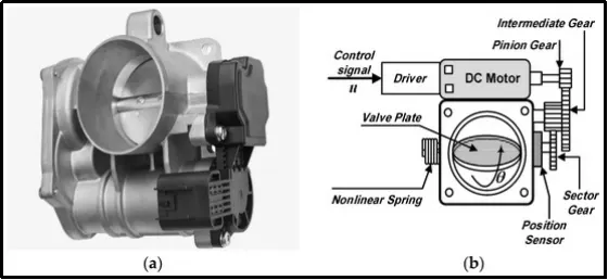
• A throttle valve is a valve designed to regulate the supply of a fluid (as steam or gas and air) to an engine and operated by a handwheel, a lever, or automatically by a governor.
• Especially it is the valve in an internal-combustion engine incorporated in or just outside the carburetor and controlling the volume of vaporized fuel charge delivered to the cylinders

Geometry Cleanup:-

To start the simulation, geometry cleanup is necessary. As we require the only fluid region to simulate fluid flow, we have to modify our geometry as per our simulation setup.

Before simulation import, the actual model of the throttle valve in the converge by just drag and drop method. Even before importing the geometry, prior check the geometry in ".stl", ".step" or ".iges" format. As those are the universal cad accepted formats for all the software.

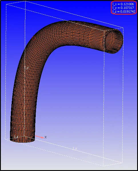
After importing the geometry, it is good practice to check the geometrical dimension and geometry bounding box. Converge only accepts the dimension in meters. So even if the geometry was made using millimeters by previous software converge only accept it as a meter.

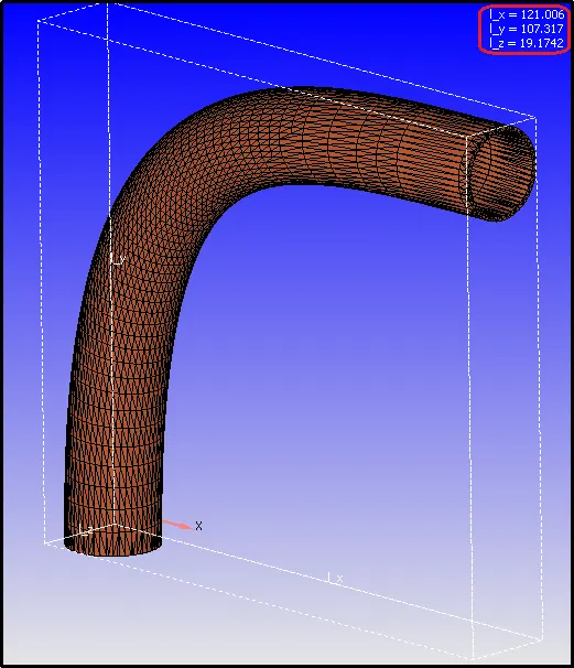
By using the scale option available in converge, we can reduce the size of the entire geometry at one click. so the above geometry size was reduced using a 0.001 scale factor.

Boundary Definition:-

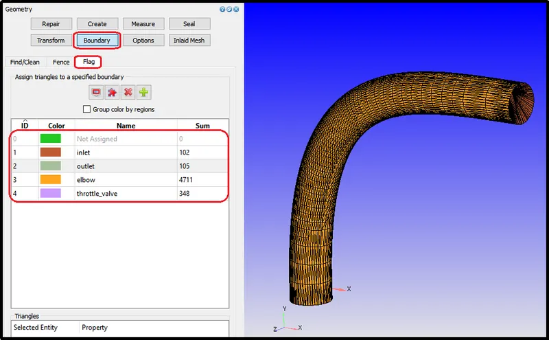
In boundary definition, first, add the number of boundaries as per requirement. In this particular case, we require 4 boundaries. Later, assign that boundary to a separate surface.

And finally rename the boundary as per the relative boundary type - Inlet, Outlet, throttle Wall, and Elbow Wall.

Geometry Diagnosis:-

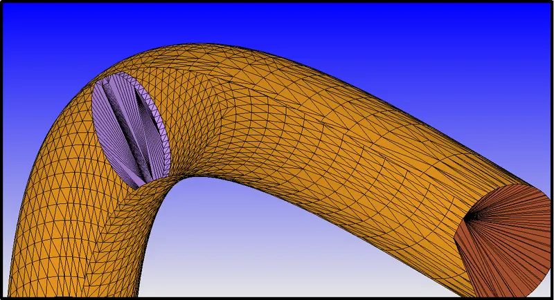
By using the hide option, we can hide selected elements in the converge, which is a useful tool to examine the internal part of the geometry. In this specific case, we need to check the boundary assignment for the throttle valve.

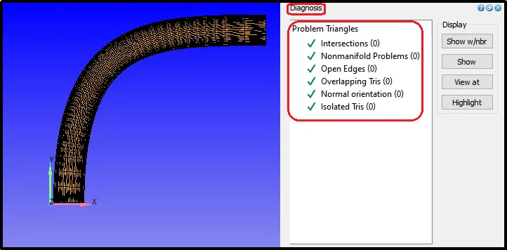
Lastly, using Diagnosis check all the geometry setup is ok or not. Here it checks intersections, Non-manifold Problems, open Edges, Overlapping tris, Normal orientation, and Isolated tris.

Simulation Setup/ Case setup:-

Application type:-

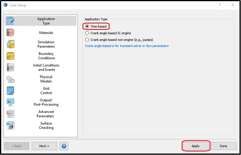
In the 'Application Type" section selects the "Time-based" application and click apply and done. later, we will get the option for a steady flow solver. It will show us a setup tree.

Material Definition:-

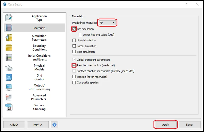
In this simulation, we simulated the results for compressible flow with fluid air.

Simulation Parameters:-

Run Parameters:-

This is a steady-state simulation, so the steady-state solver type was selected with simulation mode Full hydrodynamic using gas flow solver as compressible.

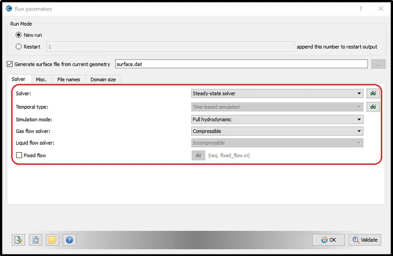
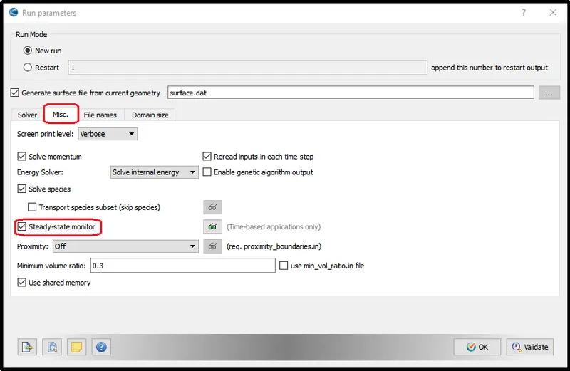
To monitor our results and converge our results with proper tolerance, the steady-state monitor box was checked. This gave us the option to control the accuracy of our results.

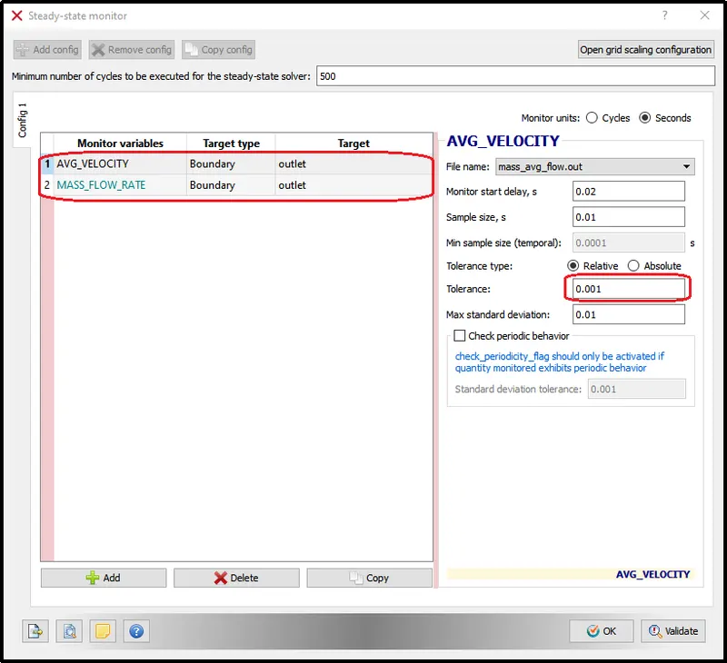
Steady-state monitor:-

In Steady-state monitor input two-parameter were monitored - one was Velocity at the outlet and another was mass Flow rate at the outlet. Tolerance for both was set as 0.001.

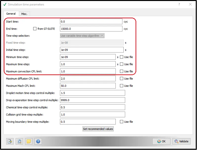
Simulation time parameters:-

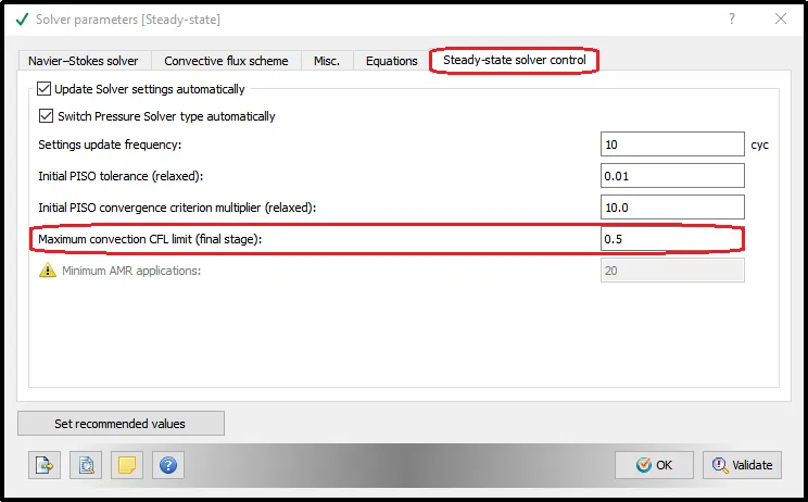
The cycle range was set for 0 - 15000 cycles with the initial time step and a minimum time step of 1e-09. Value of maximum time-step and maximum convection CFL limit set for 1.

Solver Parameters:-

In the solver Parameter, it is very important to set Maximum convection CFL limit control below 1. For this simulation is set as 0.5

Fluid Region:-

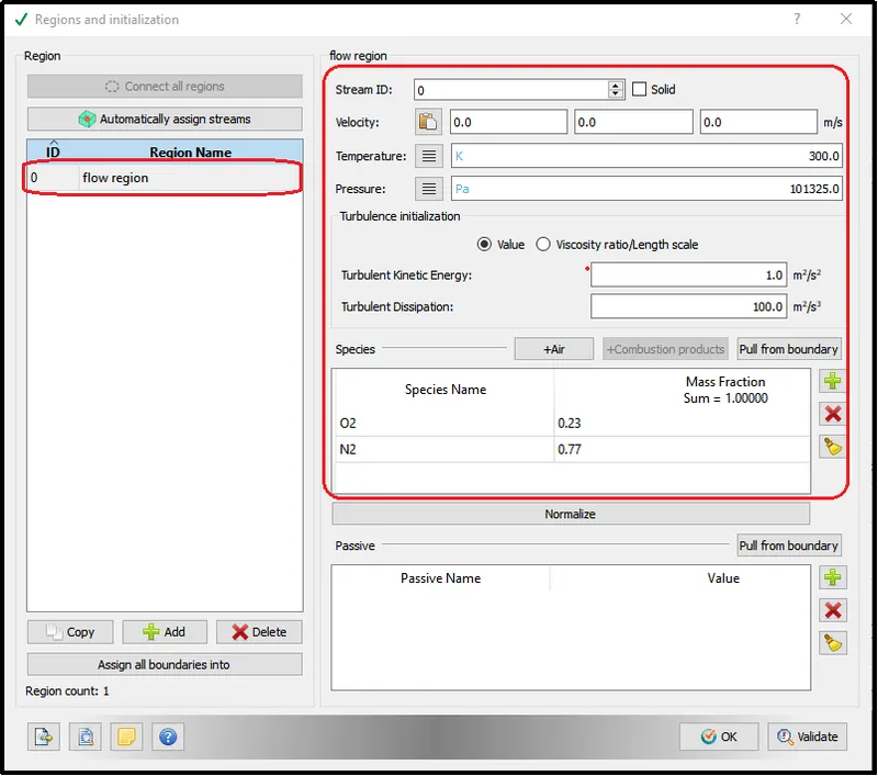
Apart from the boundary surface, cells also generate in the inner volume. Therefore, it is important to assign some material or fluid material with particular property conditions to these cells.

So, we define it as a flow region with material fluid as air with normal pressure and temperature at its initial state.

Boundary Conditions:-

Inlet:-

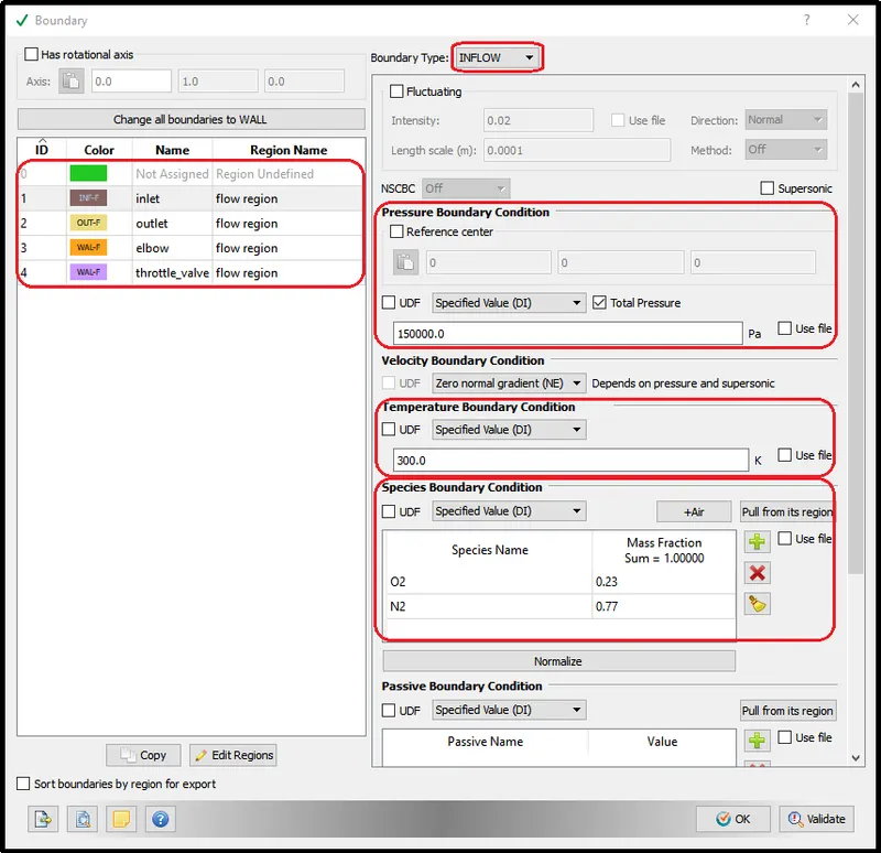
At the inlet, we are giving a pressure of 1.5 bar with a 300k temperature as an air inlet.

Outlet:-

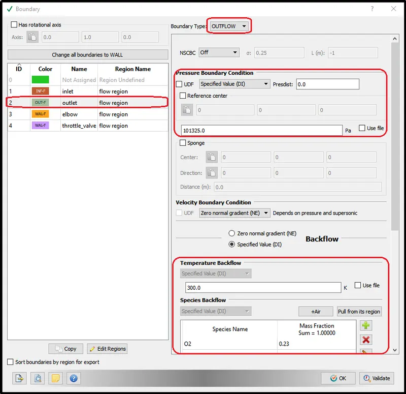
At the outlet, normal atmospheric pressure and temperature conditions are considered.

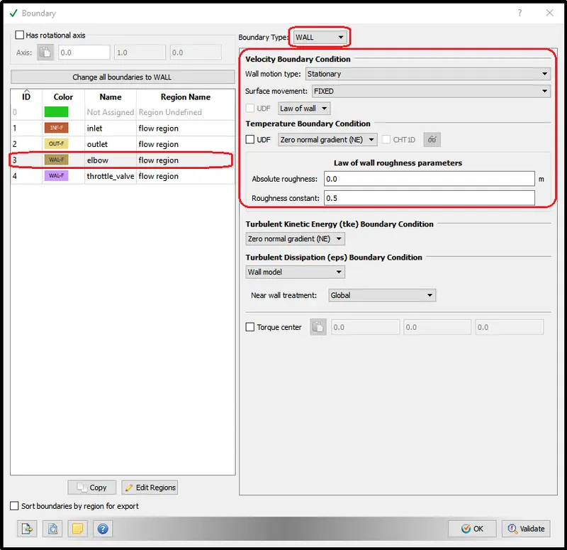
Elbow wall:-

The Elbow wall is the casing wall so it will be at stationary condition fixed surface. with normal law of wall condition.

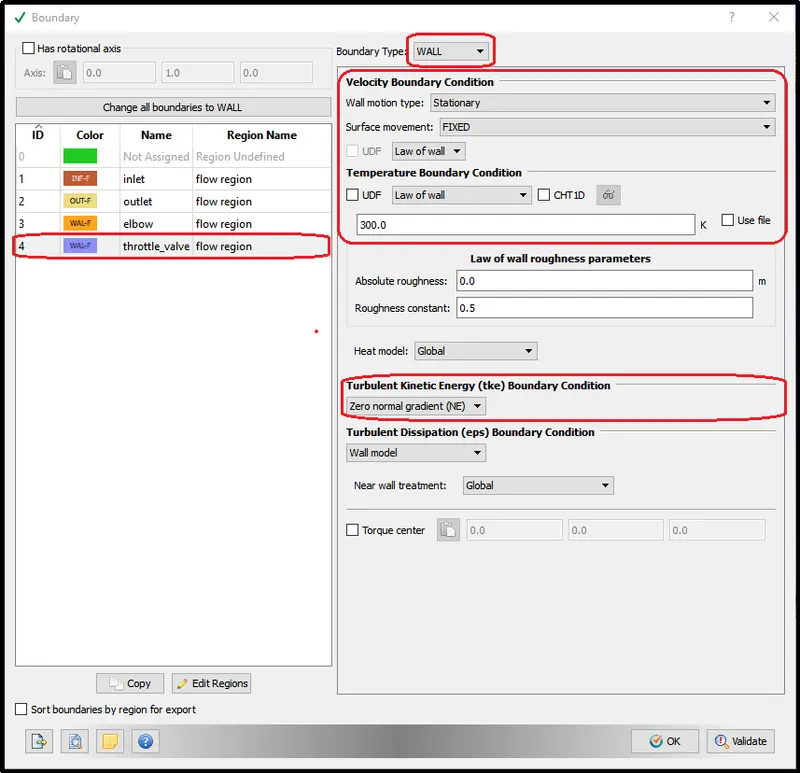
Thottle_valve:-

In a Steady-state condition, the flow does not change with respect to time. so there is no point to give wall movement according to time. As for the mentioned condition, we can only get the final result for any case. so here we consider throttle wall is fixed and obeying the Law of wall surface condition.

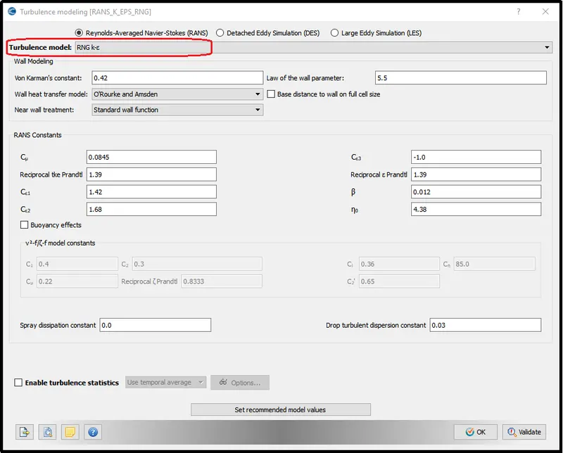
Turbulence model:-

Here, the turbulence model was used as RNG K-epsilon. because because of obstacle or throttle valve the laminar stream converted into turbulent.

Grid Control/ Meshing:-

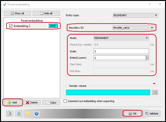
In the 'Grid Control' setting add the "fixed embedding" parameter.

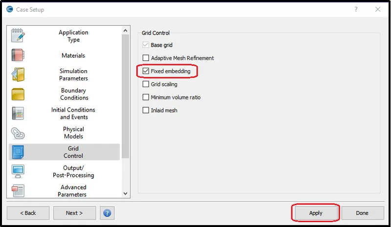
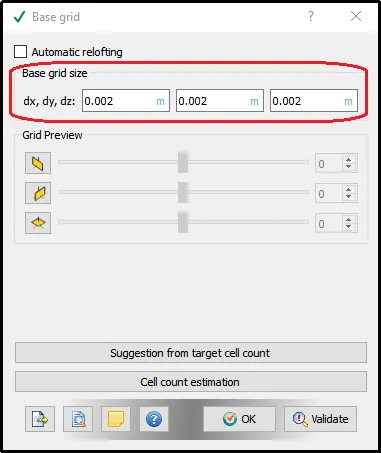
The grid size of 0.002m was given to all the directions.

Near throttle wall surface fine mesh si required to capture accurate fluid flow near the throttle wall. The density of the cell near the throttle will give a clear representation of flow change near the throttle wall.

so the scale was used 3 with embedded layers of 2.

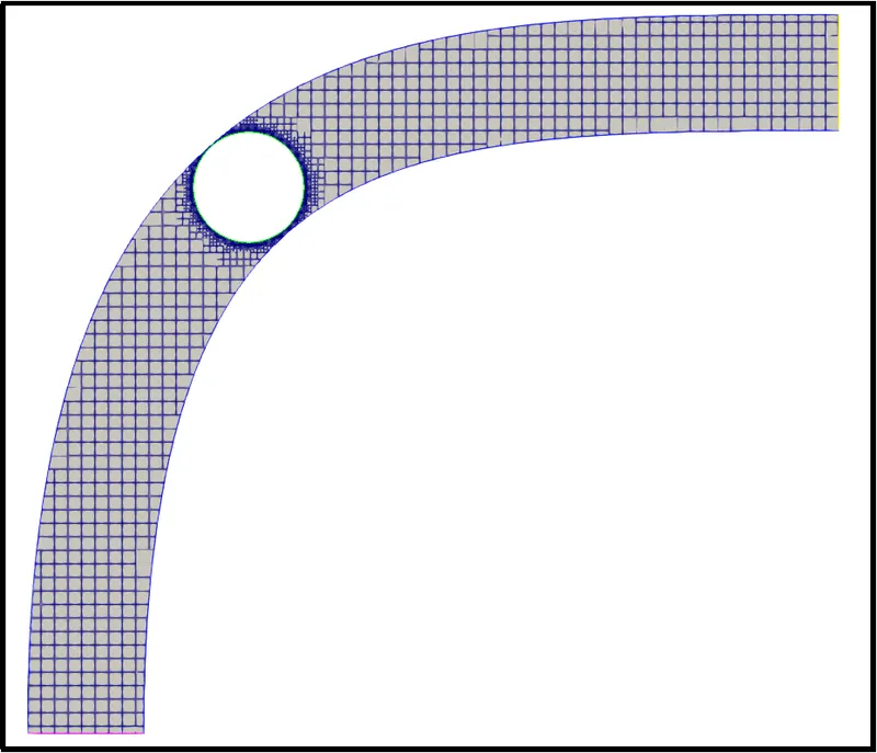
The mesh over the geometry looks like this after using the above setting parameters.

Output/Post-processing:-

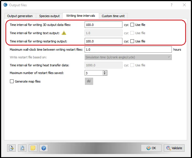
The time interval for writing 3D output data files is kept for 100 cycles i.e. after 100 cycles it will create one 3D output file.

The time interval for writing restarting output was also kept for 100 cycles which will help us restart the simulation in the last count of 100 cycles in case simulation stopped unexpectedly. It helps to save the simulation time of the user.

Complete Case setup:-

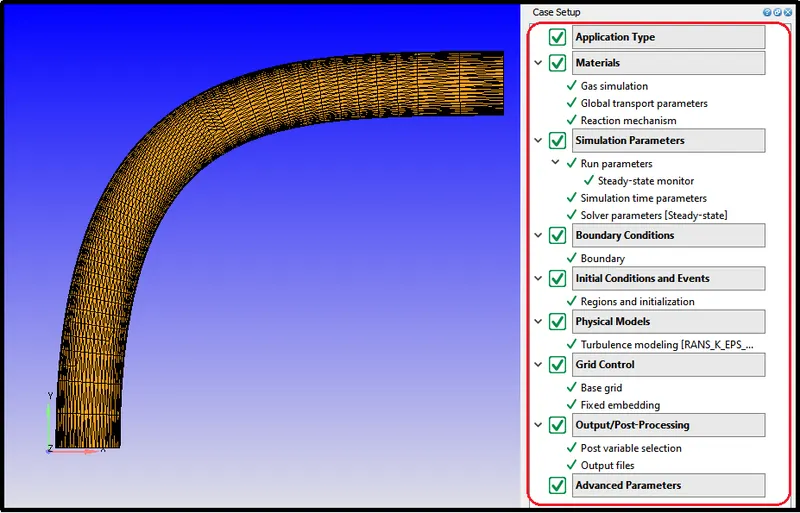
Converge shows a good representation of the completion of each case setting. It shows that the setup is correct by representing a green checkmark as portrayed in the below figure.

Export Input files:-

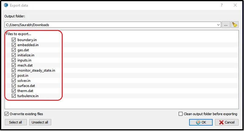
Using file -> Export -> Export Input files all the input files were exported to the simulation folder.

Simulation Run:-

The simulation was run with the help of Cygwin. The directory contains all the export files that were located and using the ‘converge.exe’ setup the simulation was run.

Convergence plots for Average Velocity at Outlet:-

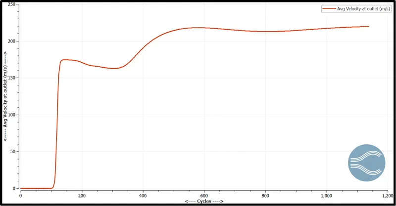
The following graph shows the variation of velocity as the number of cycles increases. It exhibits that the Simulation is converging at the 1138^th cycle. From the 1100^th cycle its showing constant average velocity at the outlet of the throttle valve.

Convergence plots for Pressure at outlet:-

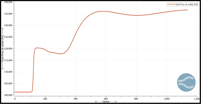
If we observe pressure charts like velocity pressure also slowly giving constant value as cycles move forward.

Convergence plots for Mass Flow rate at the Inlet and Outlet:-

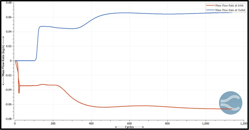
The line graph provides the information of mass flow rate at the inlet and the outlet as per the increment rate of simulation cycles. From 1100th cycles the mass flow in and mass flow out giving constant results which means that the results are properly converged.

Total cell count:-

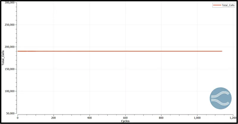
For the steady flow, there is no movement in the throttle valve so there will be no new mesh generation process as the geometrical shape of the fluid region remain the same in the overall simulation and, therefore, the cell count will be also the same for the overall simulation. The overall cell count we are getting for the simulation is 189979 number cells.

Velocity Contour:-

The following figure illustrates the velocity contour with velocity vector over the mid surface along the Z-direction. As the flow is steady there is no movement in the throttle valve so the throttle valve remained stationary for all the cycle.

At the turning of the elbow pipe, the velocity slightly increases.

Afterward, the velocity strikes the throttle body which devices the velocity streams into two parts. This is responsible for the pressure drop which increases the velocity near the outlet of the throttle valve.

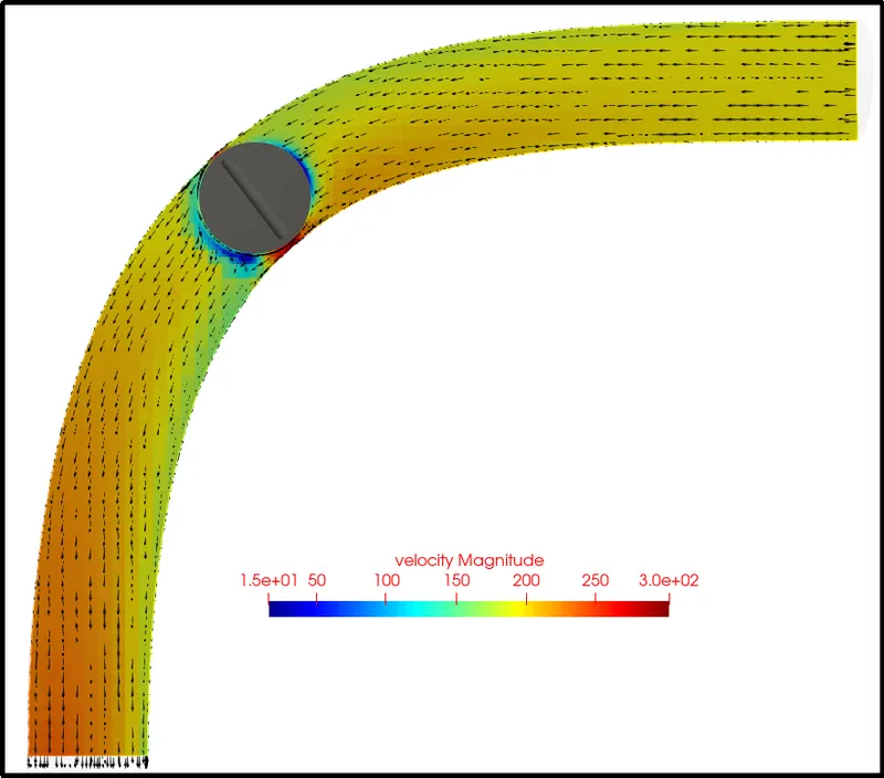
The velocity of the fluid (air) strikes on the valve body which is responsible for the high pressure on the front side of the body and at the back part because of less aerodynamic shape eddies form near the back surface of the valve. which is responsible for the lowest pressure on the valve body. To get closer observation next we will take a look over the pressure contour plot.

Variation in velocity with increment in cycles:-

In the below video, we can see the convergence of velocity - how velocity reached its steady-state with the increment of the no of cycles.

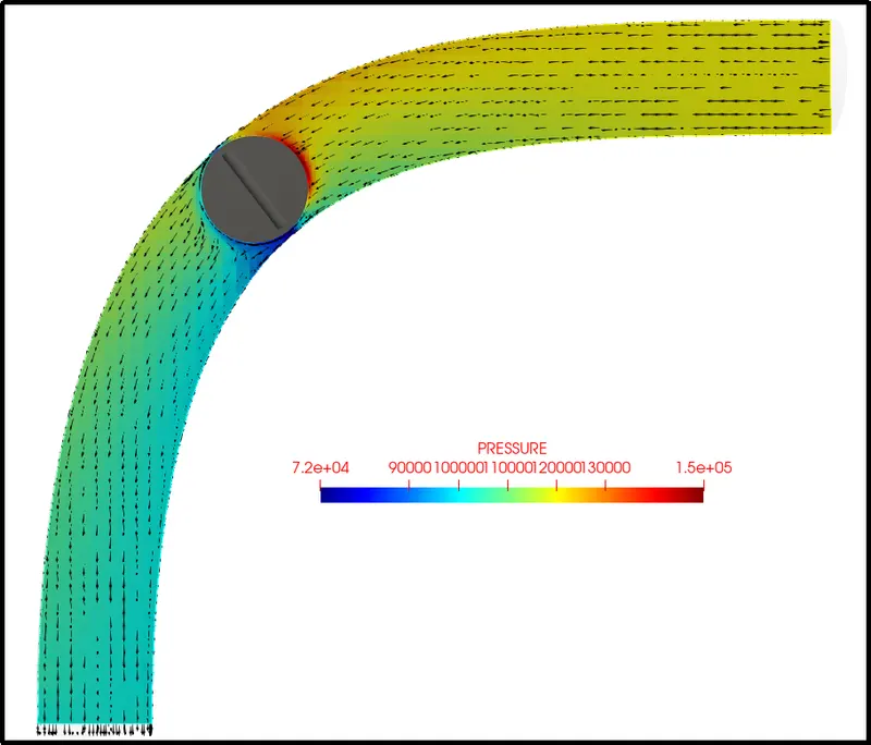
Pressure Contour:-

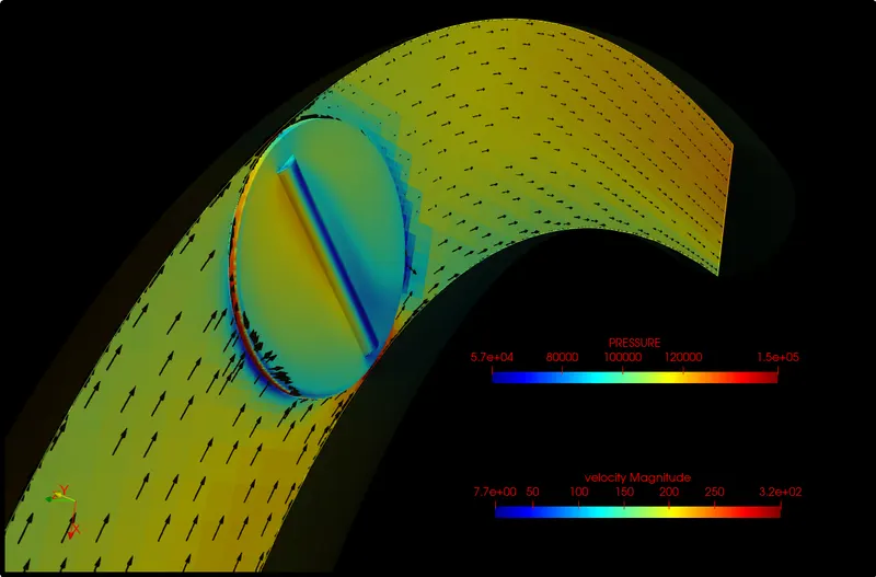
The following figure portrays the representation of pressure on the mid surface of the throttle valve body. Here, we can observe the pressure from the inlet is decreasing slowly. this happens because of the wall friction. One can notice, loss of pressure starts to increase more at the turning area of the elbow section.

Then the air stream strikes the throttle valve responsible for the generation of high pressure at the front part of the throttle valve. On the contrary, we can see eddies formation at the end of the throttle valve which is responsible for the low-pressure region.

In this case the throttle plate act as an obstacle that leads to the pressure drop and increases in velocity of the air.

Variation in pressure with increment in cycles:-

In the below video, we can see how pressure reached its steady-state with the increment of the no of cycles.

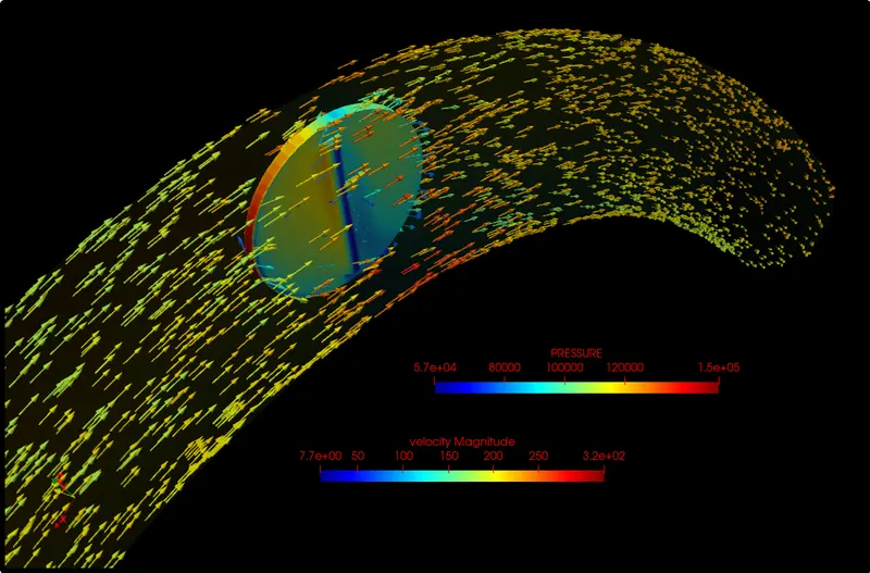
Vectors of the flow stream velocity:-

With below picture of the vector 3D plot, we can see how fluid strikes on the surface of the throttle valve and create different pressure effect over the surface of the throttle valve.

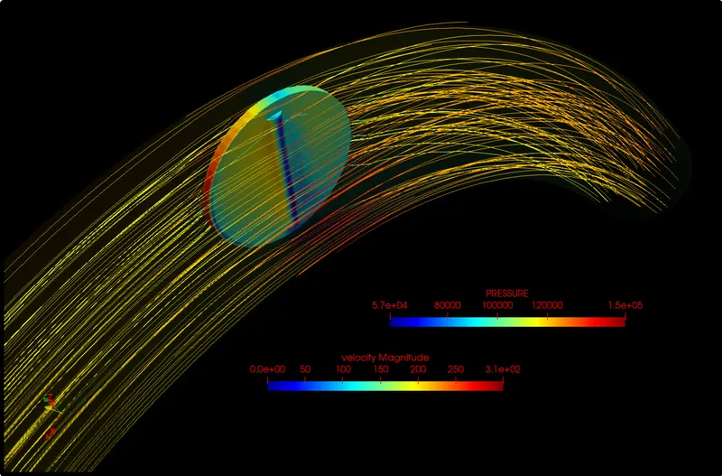
Streamline Flow over the Valve body:-

With the streamline flow picture of the model, we can notice how the laminar streamline flow changing into the turbulent flow and how the fluid flowing around the surface of the valve body.

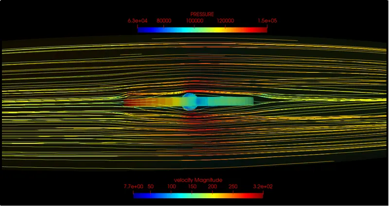
Below the image is the top view of the throttle valve which shows how sir strikes on the valve body and how streamlines divide by the valve when the valve is open

Change in streamline flow as per simulation cycles:-

In the below video, we can observe the changes in streamline flow with the increment of simulation cycles. The flow slowly reaches its steady state.

As this is a steady-state simulation, we cannot observe the throttle movement in the simulation. Because the throttle movement is defined by the time and in steady-state simulation the setup is not time dependant. Here, results are constant or do not change with respect to time.

Observation:-

The observation table is the final max and min value we got from this steady-state simulation. later we will compare it with the transient state simulation values to check the differences in results and to validate them.

Conclusion:-

• Geometry cleanup is important to set the required fluid domain for the simulation.
• Fixed embedding is a great tool to refine mesh near the required surfaces of the parts.
• Pressure drops because of friction near the turning section of the elbow pipe and the lowest pressure is observed near the end side of the Valve surface where eddies form.
• As the pressure drops because of the throttle valve acting as an obstacle velocity near the outlet area starts to increase which obeys Bernoulli's principle which is the principle of conservation of energy.

Project Link:-