EXAMINING STABILITY OF AN ORDINARY DIFFERENTIAL EQUATION BY CONSIDERING IMPLICIT AND EXPLICT SCHEMES

Aim :

1. To understand the reason for unstabilty
2. To figure out which scheme stands stable for larger time steps

Theory :

A numerical method is said to be unstable if small perturbations cause the solution to oscillate and diverge

consider the ODE

`f(y)=(dy)/dx=-1000y-e^(-t)`

Here two schemes are considered implicit scheme and the explicit scheme. In explicit scheme the values of the previous time step are used for computation and in implicit schemes the values from the current time step are used and hence iterative techniques are used

Eulers forward difference (Explicit scheme) :

`y_(n+1)=y_n+hf(y_n,t_n)`

`y_(n+1)=y_n+Deltat(-1000y_n-e^(t_n))`

`y_(n+1)=y_n-1000y_nDeltat-e^(t_n)Deltat`

`y_(n+1)=y_n(1-1000Deltat)-Deltate^(t_n)`

here

`(1-1000Deltat)` is a growth factor

if `|1-1000Deltat|le1`the solution is stable

if `|1-1000Deltat|>1`the solution becomes unstable

From this relation the value of time step can be determined

The above stability condition represents the equation of a complex representation of a circle with radius 1 and center -1

For the explicit scheme to be stable `-1000Deltat`should lie inside the circle

Euler's backward difference (Implicit scheme) :

`y_n=y_(n-1)+hf(y_n,t_n)`

`y_n=y_(n-1)+Deltat(-1000y_n-e^(t_n))`

`y_n=(y_(n-1)-Deltate^(t_n))/(1000Deltat+1)`

`|1/(1+Deltat1000)|le1`is the stabilty criterion . This extends to the entire left complex plane and hence it has wide range of stability

Analytical solution :

`y(t)=(e^(-1000t)(1-e^(-999t)))/999`

python code :

import numpy as np
import matplotlib.pyplot as plt
import math

def explicit_euler(total_t,dt):
	t=np.arange(0,total_t,dt)
	y=np.zeros(len(t))

	for i in range(1,len(t)):
		y[i]=y[i-1]+dt*(-1000*y[i-1]-np.exp(-t[i-1]));

	return[t,y]


def implicit_euler(total_t,dt):
	t=np.arange(0,total_t,dt)
	y=np.zeros(len(t))

	for i in range(1,len(t)):
		y[i]=(y[i-1]-np.exp(-t[i-1])*dt)/(1+1000*dt)

	return[t,y]

def analytical(total_t,dt):
	t=np.arange(0,total_t,dt)
	y=np.zeros(len(t))

	for i in range(1,len(t)):
		y[i]=np.exp(-1000*t[i])*(1-np.exp(999*t[i]))/999

	return y

total_t=0.1
dt=1e-4
t,y_explicit=explicit_euler(total_t,dt)
t,y_implicit=implicit_euler(total_t,dt)
y_analytical=analytical(total_t,dt)
plt.plot(t,y_explicit,color='blue')
plt.plot(t,y_implicit,color='red')
plt.plot(t,y_analytical,color='black')
plt.legend(['explicit','implicit','analytical'])
plt.show()

Output :

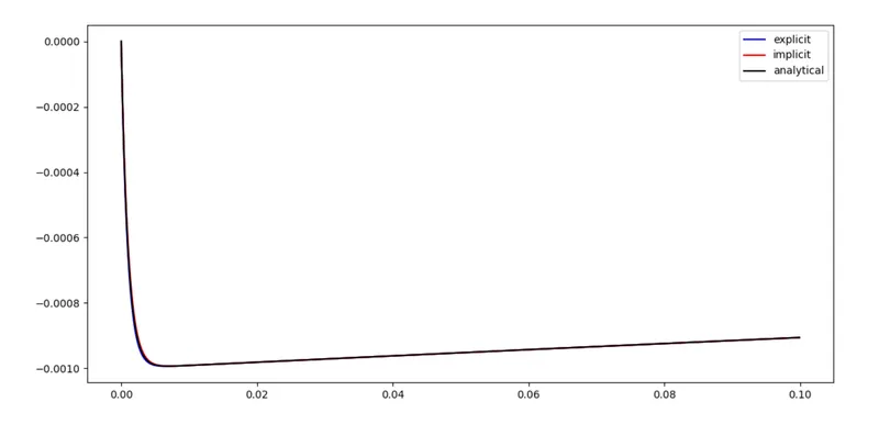
for dt = 1e-4

for dt = 1e-3 :

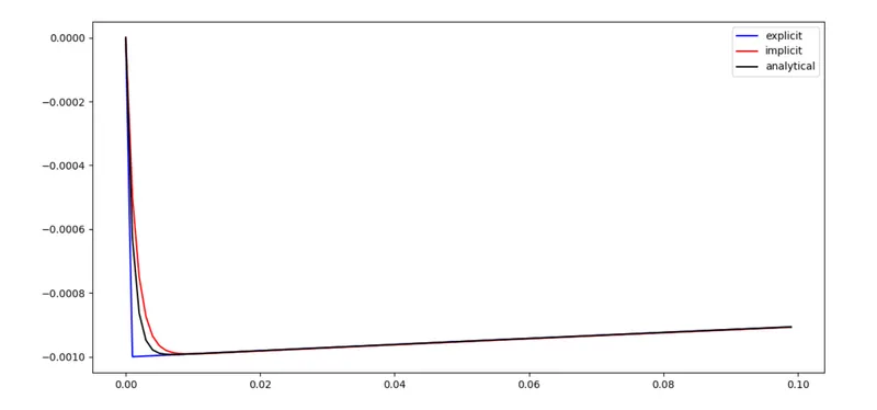
A sharp edge has appeared in the explicit solution which means the solution is ready to blow up

For dt = 2e-3 :

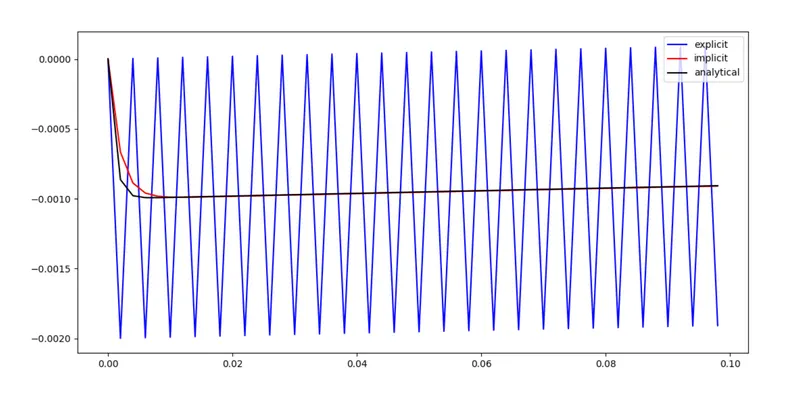
The explicit solution has blown up and the implicit solution still gives the accurate solution

For dt =1e-2 :

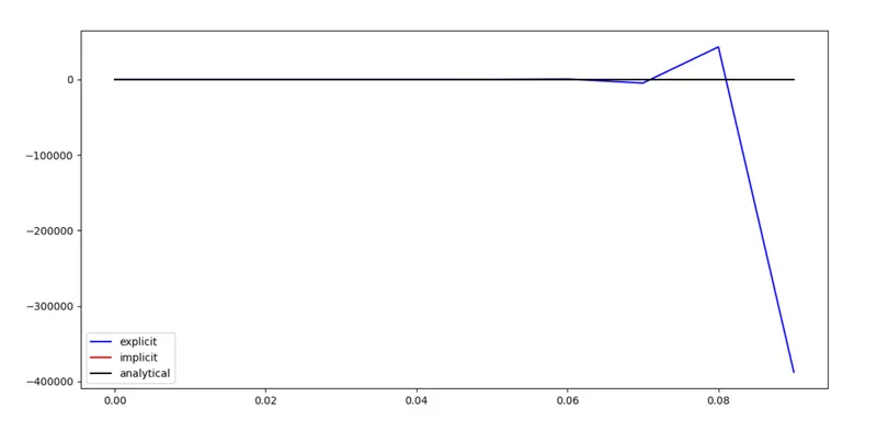
The explicit solution has blown up completly

Conclusion :

1. For larger time steps explict scheme becomes unstable
2. It is always bad to have an unstable solution for any kind of engineering simulation as it gives unphysical results
3. Eigen value analysis and von-neumenn stability analysis determine the stability condition for all types of problems.