Simulink SIMULATION OF SHAPING MACHINE WORK DONE, EQUATION Modeling AND SPRING MASS DAMPER SYSTEM Models COMPARISION

AIM:

To make a Simulink model for evaluating shaping machine work done, equation solver and spring mass damper system comparison.

OBJECTIVES :

1. Generate a Simulink model for evaluating work done by a shaping machine.
2. Generate a Simulink model to solve a given equation with multiple variables.
3. Comparison of Spring Mass Damper system using Simulink and Simscape.

EVALUATING WORK DONE BY A SHAPING MACHINE

INTRODUCTION :- To evaluate the work done using the given parameters of a Shaping Machine Cutting Tool,

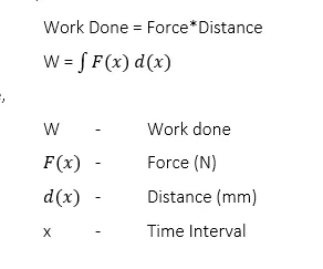
BLOCKS USED :-

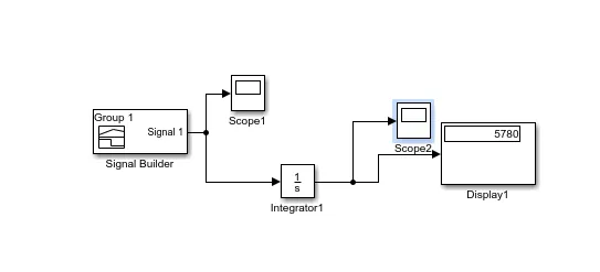
1. signal builder Block – To send the distance and force values.
2. Integration Block – To integrate both distance and force values for obtaining the work done value.
3. Display Block – To view the work done value.
4. Scope – To plot two different data sets for better understanding.

SIMULINK MODEL :-

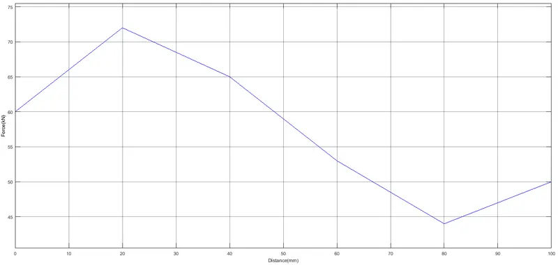
Input:

steps:

1. Initially the distance (mm) and force (KN) is inputted through signal builder block
2. Next both distance (mm) and force (KN) are integrated to evaluate the work done values.
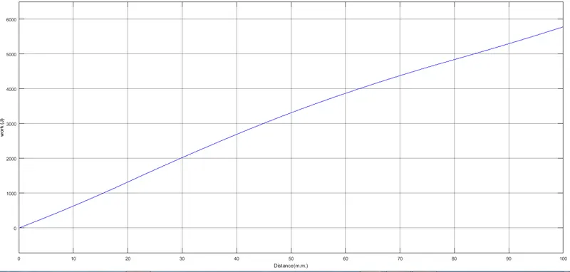
3. Finally, the work done and distance graph is plotted.

output:

GENERATE A SIMULINK MODEL TO SOLVE A GIVEN EQUATION WITH MULTIPLE VARIABLES:

INTRODUCTION :-

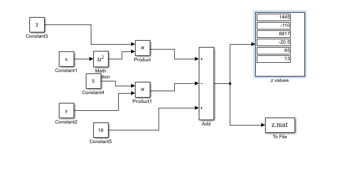
To solve the following equation by inputting various values from array datasets as follows:

`z = 3x^2-5y+18``

BLOCKS USED :-

1. Constant – To represent the values of ‘3, 5 & 18’.
2. Subtract – For solving the equation.
3. Square – For squaring the input
4. Product – To evaluate and generate the function output.
5. Display – To show the evaluated value.
6. To File – To save the evaluated values w.r.t time interval.

Model:

Steps:

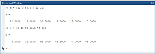
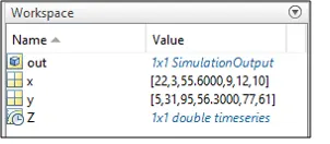
• Initially the array datasets to be inputted in the workspace for both ‘x’ and ‘y’ variables
• Next the first value from ‘x’ dataset will be taken and squared then multiplied by 3 to get the value of 3x^2.
• Then the first value from ‘y’ dataset will be taken and multiplied by 5 to get the value of 5y.
• Then the final equation is solved and the values are displayed.
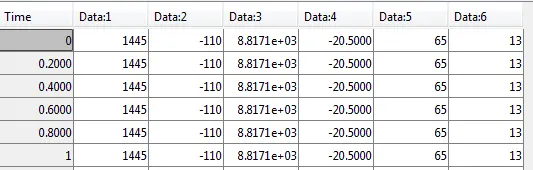
• Finally the saved values are stored in ‘Z.mat’ file.

VERIFICATION CALCULATION :-

For x=22,y=5

z=3*(22^2)-5*5+18=1452-25+18=1445

Output :-

The equation for all the values from the dataset are solved and stored in ‘.mat’ format file. Here we ran the simulation 10 sec so we can conclude that the same value is obtained for many iterations of the simulation though 0.2 seconds time steps.In the figure below only the first second is shown

COMPARISON OF SPRING MASS DAMPER SYSTEM USING SIMULINK AND SIMSCAPE:

BLOCKS USED :-

1. Gain Block – To multiply with constant value to the input given
2. Subtract – For solving the equation.
3. Integrator block – To integrate the velocity and distance values
4. Goto Block – To send the signal from any subsystem or in main model to any place
5. From Block – To receive the sent signal from Goto Block
6. Scope – To plot graph between two parameters
7. Ideal Translational Motion Sensor Block – To sense the movement (velocity) of the system
8. Damper, Spring, Mass Block – To model a spring mass damper system
9. Mechanical Reference – To make sure that all the components are clamped to the ground
10. Solver Configuration – It specifies the solver parameters before starting the simulation
11. Mux block:Combine input signals of same data type and complexity into virtual vector
12. ps simulink converter:to convert physical signal to simulink signal
13. Simulink ps converter:to convert simulink signal to physical signal
14. clock block-It outputs the current simulation time at each simulation step
15. To Workspace block:writes data to workspace

SIMULINK & SIMSCAPE MODEL (ORIGINAL Model) :-

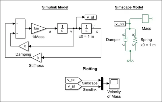
steps simulink:

1-The mass (m), spring constant (k), damping co-efficient (b) variables are inputted from the MATLAB workspace window

2-while the original displacement (x0 = 1) is inputted from integrator block

3-Then acceleration a is calculated by `a=1/m*(-b*v-k*x)`

4-Then it is integrated to get velocity and then integrated again to get the displacement

5-Then simscape and simulink signals are sent via Goto and from block to the scope and then combined into one signal using the Mux block to enter the scop through one input

Steps simscape:

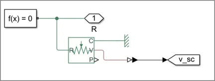
Th same as simulink but it has uses transational reference and motion sensing block to measure the velocity of the mass,it takes input from r while c is reference and the output is via velocity port which is converted to simulink signal vis ps simulink converter

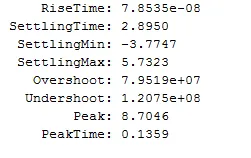
Signal Chracteristics Definitions:

Measuring signal characteristics:

steps:

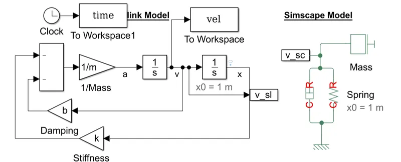
1-using clock block that is connected to "TO workspace block" the time can be sent to the workspace

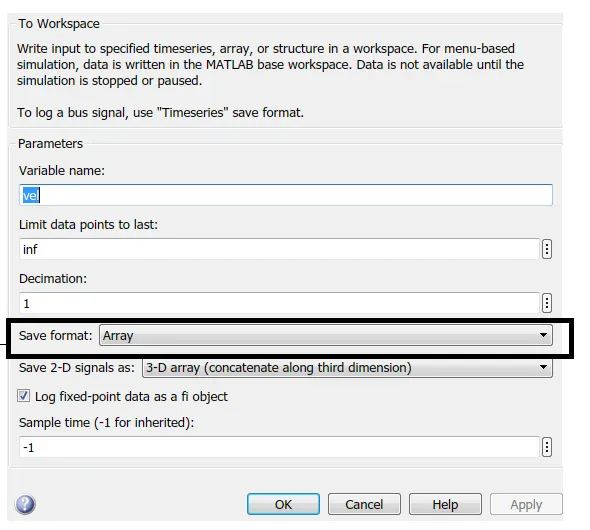
2-Then another "To workspace" block is used to save the output velocity values to the workspace

3-In the"To workspace" block parameters change the save format from Time series to an "Array"

4-Then using "stepinfo" command in matlab,all the transient time data can be obtained

Initial output:

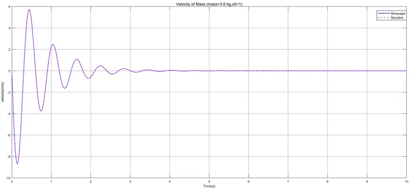
Initially both model have the same output

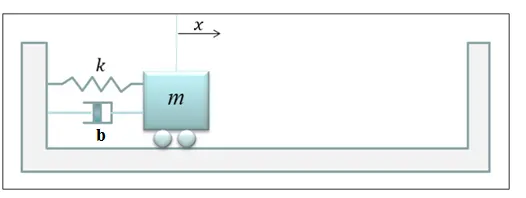
TASK I - DERIVATION OF GOVERNING EQUATION :-

In this model we are using Spring Mass Damper System with Simple Harmonic Motion.

From Newton’s Second Law of Motion,

`F = m*a`

The restoration force of spring i.e., returning to equilibrium position,so i

`Fsp = kx`

The damping force in the system

`Fd = b*v=b*dx/dt`

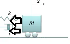
looking at the free body diagram it appears that the spring and damper forces acting in the negative direction compared to the displacement then replacing F in first equation:

so

`-Fsp-Fd=ma`

so `ma+fd+fsp=0`

so `ma+bv+kx=0`

Inorder to put all the equation in the x variable:

`a = (dv)/dt`

and `v=dx/dt`

Now,

`a = (dv)/dt`

`a = (d/dt)*v`

`a = (d/dt)(dx/dt)`

`a = (d^2x)/(dt^2)`

WKT,

`F = m*a`

`F = m*(d^2x)/(dt^2)`

By equating,

`F = m*a`

`-kx-bdx/dt = m(d^2x)/(dt^2)`

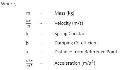
`m(d^2x)/(dt^2)+bdx/dt+kx = 0`

TASK II – CHANGING THE PARAMETERS IN SIMSCAPE MODEL:

The parameters being changed in the Simulink model are mass (m), damping co-efficient (b), spring cons and then plot the results.All the parameters will be multiplied by a 2.7 factor,so the new mass will be 10 kg and new k will 1080n/m and new b will 27 ns/m

changing the mass result:

mass was changed from 3.6 to 10 kg

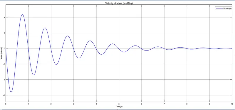
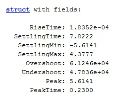
It can be noticed that the settling time has increased from 2.8 s to 7.8 s while the peak value was reduced from 8.7 m/s to 5.6 m/s

changing the spring constant k result:

k was changed from 400 N/m to 1080 n/m

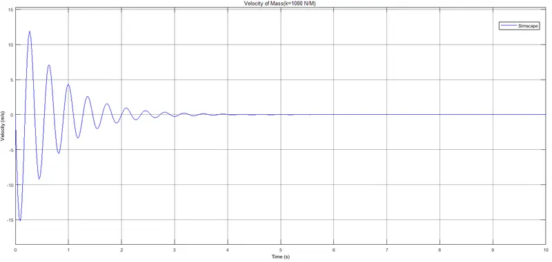
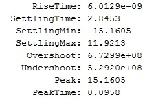
It should be noted that increasing spring constant didn't change the settling time but resulted in increased peak value from 8.7 m/s to 15.1 m/s

Changing the damping coefficient b result:

Damping coefficient was changed from c=10 ns/m to c=27 ns/m:

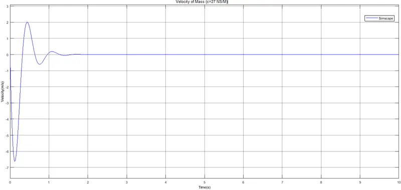
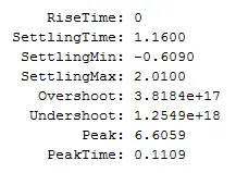
increasing the damping coefficient reduced the settling time from 2.8 s to 1.16s and reduced peak value from 8.7 m/s to 6.6 m/s

TASK III – CHANGING THE PARAMETERS IN SIMULINK MODEL :-

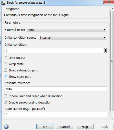
The simulink model uses the initial conditions implemented via the integrator block (x0)

the parameters of the mass and x0 are changed in the simulink model from 3.6 kg and 1m to 10 kg and 2 m

the mass can be changed from the workspace in matlab while the x0 can be changed from the integrator parameter configurator window:

Results:

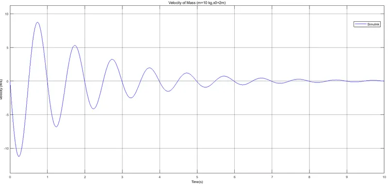
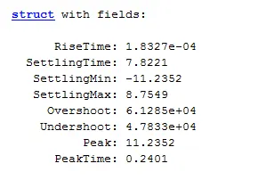
It should be noted that increasing the displacement from 1 to 2 m didnt affect the settling time for mass of 10 kg which remained at 7.8 second (as previously shown in the simscape model),it only increased the peak value from 5.6 to 11.2 m/s

TASK IV –MAKING SIMSCAPE AND SIMULINK AS TWO SEPARATE DISPLAYS :-

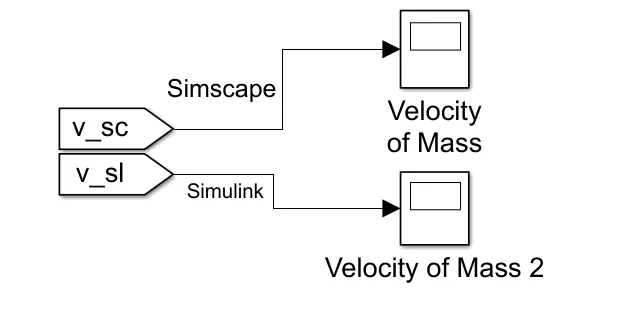
Removing the mux block will allow us to take the output of each signal to a separate scope:

CONCLUSION :-

The work done by shaping machine, solving the equation with array dataset and comparing the spring mass damper system with Simulink and Simscape was completed successfully

Reference:

Matlab help

Models:

First model:

https://drive.google.com/file/d/1U8vXrXbv2Dr70TuknMjyUCTddibcbtgU/view?usp=sharing

second model:

https://drive.google.com/file/d/1RIVlsP-nPe1VmKB1Lfxwj9CWzGkD6bMT/view?usp=sharing

output file (z values) second model:

https://drive.google.com/file/d/1pbHZiAZdGwUH1wAmQ1n8hXhdaQYQyQcI/view?usp=sharing

Edited third model:

https://drive.google.com/file/d/1TJRGpbj5OjXi409_V5g5fxSNiuzHxT53/view?usp=sharing