Simulation of Flow through a pipe in OpenFoam
Simulation of Flow through a pipe in OpenFoam
Objective :-
- Reynolds number based on pipe diameter and inlet velocity should be 2100
- Working fluid - water
- You need to calculate the length of the pipe
- Calculate length of the pipe using the entry length formula for laminar flow through a pipe
- Show that entry length is sufficient to produce a fully developed flow. You will have to compare velocity profiles at different positions along the length of the pipe.
- Solver - icoFOAM
- Write a program in Matlab that can generate the computational mesh automatically for any wedge angle and grading schemes
- Hint: wedge angle should be less than 5 degrees
- Make sure that number of cells along the "axi symmetric"
- For a baseline mesh, show that the velocity profile matches with the Hagen poiseuille's equation
- Show that the velocity profile is fully developed
- Post process velocity and shear stress
Hagen-Poiseuillie Equation :-
The law states that the flow of liquid depends on following factors like the pressure gadient (Δp) the length of the narrow tube (L) of radius (r) and the viscosity of the fluid () along with the relationship among them.
Hagen-Poiseuille equation Continuum mechanics. To calculate the flow through each lamina, we multiply the velocity from above and the area Poiseuille the lamina. Finally,pu this expression in the form of a differential equation dropping the term quadratic in dr . The assumptions of the equation are the fluid is incompressible and Newtonian; the flow is laminar through a pipe is constan circular cross-section that is substanially longer that its diameter; and there is no acceleration of fluid in the pipe.
- The Pressure Gradient (Δp) Shows the difference in the pressure between the two ends of the tube, determined by the fact any fluid will always flow from high pressure (p1) to low pressure region (p2) and the flow rate is determined by the pressure gradient (P1-P2)
- Radius of tube the liquid flow varies directly withradius to the power 4.
- Visocosity () The flow of the fluid varies inversely with the viscosity of the fluid and as the viscosity of the fluid increases, the flow decreases vice-versa.
- Length of the Tube (L) the liquid flow is inversely propostional to the length of the tube therefore longer than tube greather is he resistance to the flow.
- Resistance (R) the resistance is described by 8Ln/pir4 and therefore the Poiseuillie's law becomes
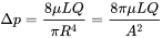
where:
- Δp is the pressure difference between the two ends,
- L is the length of pipe,
- μ is the dynamic viscosity
- Q is the volumetric flow rate,
- R is the pipe radius,
- A is the cross section of pipe.
The Equation are that the fluid is incompressible and Newtonian the flow laminar through a pipe of constant circular cros section that is substainly longer than is diameter and there is no acceleration of the fluid in the pipe .For velocities and pipe diameter above the threshold actual fluid flow is not laminar but turbulent.leading to larger pressure drops then calculated by the Hagen-Poiseullie equation.
The analytical calculation to obtain initial condition as geometric are:
- Fluid ; Water
- Reynolds number : 2100
- Kinematic Viscosity: 0.475e^-6
- Density :983.2Kg/m^3
- Diameter: 0.127m
- Solver : icoFoam
When the fluid just enters the pipe, the thickness of the boundary layer gradually increases from zero moving in the direction of fluid flow and eventually reaches the pipe center and fills the entire pipe. This region from the entrance of pipe to the point where the boundary layer covers the entire pipe is termed as the hydrodynamic entrance region and length of the pipe in this region is termed as the hydrodynamic entry length. In this region the velocity profile develops and thus the flow is called the hydrodynamically developing flow. After this region, the velocity profile is fully developed and continues unchanged. This region is called the hydrodynamically fully developed region. But this is not the fully developed fluid flow until the normalized temperature profile also becomes constant.
In case of laminar flow, the velocity profile in the fully developed region is parabolic but in the case of turbulent flow it gets a little flatter due to vigorous mixing in radial direction and eddy motio
Matlab Code :-
clear all
close all
clc

%Input
% Angle of Wedge
theta = input('enter the angle in angles');
re = 2100;
d = 0.06;
% length of the pipe
L = 0.06*re*d;
r = d/2;
% viscosity of water
mu = 0.89e-3;
% density of water
rho = 997.0;
%Kinemayic viscosity of water
nu = mu/rho;

% calculation of pressure and velocity

%average velocity
vel_avg = re*mu(d*rho);
%maximum velocity
vel_max = 2*vel_avg;
%pressure drop
del_p = (32*mu*vel_avg*L)/(d^2);
% Kinematic pressure drop
kin_p = del_p/rho;

%num of cells along the pipe
n1 = 50;
% num of celss radially
n2 = 1;
% num of cells on the curve
n3 = 300;
gfactor = 0.2;

%vertices of edge

v0 = [0 0 0];
v1 = [0 r*cosd(theta/2) -r*sind(theta/2)];
v2 = [0 r*cosd(theta/2) r*sind(theta/2)];

v3 = [L 0 0];
v4 = [L r*cosd(theta/2) -r*sind(theta/2)];
v5 = [L r*cosd(theta/2) r*sind(theta/2)];

% Printing the file
text1 ='/*--------------------------------- C++ -----------------------------------*\';
text2 ='|  =========                                                                |';
text3 ='|  \\      /  F ield         | OpenFOAM: The Open Source CFD Toolbox        |';
text4 ='|   \\    /   O peration     | Website:  https://openfoam.org               |';
text5 ='|    \\  /    A nd           | Version:  7                                  |';
text6 ='|     \\/     M anipulation  |                                              |';
text7 ='\*---------------------------------------------------------------------------*/';
text8 ='FoamFile';
text9 ='{';
text10 ='    version    2.0;';
text11 ='    format     ascii;';
text12 ='    class      dictionary;';
text13 ='    object     blockMeshDict;';
text14 ='}';

text15 ='// ************************* //';

%creating file
f1=fopen('blockMeshDict.txt',wt');

fprintf(f1,'%s\n',text1);
fprintf(f1,'%s\n',text2);
fprintf(f1,'%s\n',text3);
fprintf(f1,'%s\n',text4);
fprintf(f1,'%s\n',text5);
fprintf(f1,'%s\n',text6);
fprintf(f1,'%s\n',text7);
fprintf(f1,'%s\n',text8);
fprintf(f1,'%s\n',text9);
fprintf(f1,'%s\n',text10);
fprintf(f1,'%s\n',text11);
fprintf(f1,'%s\n',text12);
fprintf(f1,'%s\n',text13);
fprintf(f1,'%s\n',text14);
fprintf(f1,'%s\n\n',text15);

fprintf(f1,'converttoMeters 1;\n\n');
fprintf(f1,'vertices\n(\n');
fprintf(f1,'\t(%d %d %d)\n',V0(1),V0(2),V0(3));
fprintf(f1,'\t(%d %d %d)\n',V1(1),V1(2),V1(3));
fprintf(f1,'\t(%d %d %d)\n',V2(1),V2(2),V2(3));
fprintf(f1,'\t(%d %d %d)\n',V3(1),V3(2),V3(3));
fprintf(f1,'\t(%d %d %d)\n',V4(1),V4(2),V4(3));
fprintf(f1,'\t(%d %d %d)\n)\;n\n',V5(1),V5(2),V5(3));

fprintf(f1,'blocks\n(\n');
fprintf(f1,'\t hex (0 1 2 0 3 4 5 3)(%d %d %d)',n1,n2,n3);
fprintf(f1,'simpleGrading(%0.1f 1 1)\n);\n\n',gfactor);

fprintf(f1,'edges\n(\n\trac %d %d (%d %0.2f %d)\n\trac %d %d (%0.2f %0.2f %d)\n);\n\n',1,2,0,r,0,4,5,L,r,0);

fprintf(f1,'boundary\n(\n');
fprintf(f1,'\t%s\n\t{\n\t\t type %s;\n\n\t faces \n\n\t (\n\t\t\t (%d %d %d %d) \n\t\t);\n\t}\n\n','axis','empty',0,3,3,0);
fprintf(f1,'\t%s\n\t{\n\t\t type %s;\n\n\t faces \n\n\t (\n\t\t\t (%d %d %d %d) \n\t\t);\n\t}\n\n','inlet','patch',0,1,2,0);
fprintf(f1,'\t%s\n\t{\n\t\t type %s;\n\n\t faces \n\n\t (\n\t\t\t (%d %d %d %d) \n\t\t);\n\t}\n\n','pipe','wall',1,5,4,2);
fprintf(f1,'\t%s\n\t{\n\t\t type %s;\n\n\t faces \n\n\t (\n\t\t\t (%d %d %d %d) \n\t\t);\n\t}\n\n','outlet','patch',3,4,5,3);
fprintf(f1,'\t%s\n\t{\n\t\t type %s;\n\n\t faces \n\n\t (\n\t\t\t (%d %d %d %d) \n\t\t);\n\t}\n\n','front','wedge',0,3,5,2);
fprintf(f1,'\t%s\n\t{\n\t\t type %s;\n\n\t faces \n\n\t (\n\t\t\t (%d %d %d %d) \n\t\t);\n\t}\n\n','back','wedge',0,1,4,3);
fprintf(f1,');\n\n');

fprintf(f1,'mergepatchpairs\n(\n);\n\n');
fprintf(f1,'%s',text15);

fclose(f1);
Explanation :-
- To apply the wedge pipe flow euation several icoFoam simulation were processed to see the effect of shear stress, velocity gradiation, and the efficiency of the anle applied to pree processor
- By using analytical equation the initial condition as wellas the geoetry requirements by using matlab a blockMeshDict code was created being able to change several values obtain in pipe-secton of desiresd angle and length
BlockMeshDict Code :-
/--------------------------------- C++ -----------------------------------\
  =========                 |
  \\      /  F ield         | OpenFOAM: The Open Source CFD Toolbox
   \\    /   O peration     | Website:  https://openfoam.org
    \\  /    A nd           | Version:  7
     \\/     M anipulation  |
\---------------------------------------------------------------------------/
FoamFile
{
    version     2.0;
    format      ascii;
    class       dictionary;
    object      blockMeshDict;
}
// * * * * * * * * * * * * * * * * * * * * * * * * * * * * * * * * * * * * * //

convertToMeters 1;

vertices
(
    (0 0 0)
    (0 9.993908e-03 -3.489950e-04)
    (0 9.993908e-03 3.489950e-04)
    (2.520000e+00 0 0)
    (2.520000e+00 9.993908e-03 -3.489950e-04)
    (2.520000e+00 9.993908e-03 3.489950e-04)

);

blocks
(
    hex (0 1 2 0 3 4 5 3) (50 1 300) simpleGrading (0.2 1 1)
);

edges
(
    arc 1 2 (0 0.01 0)
    arc 4 5 (2.52 0.01 0)
);

boundary
(
    axis
    {
        type empty;
        faces
        (
            (0 3 3 0)
        );
    }

    inlet
    {
        type patch;
        faces
        (
            (0 1 2 0)
        );
    }

    pipe
    {
        type wall;
        faces
        (
            (1 4 5 2)
        );
    }

    outlet
    {
        type patch;
        faces
        (
            (3 4 5 3)
        );
    }

    front
    {
        type wedge;
        faces
        (
            (0 3 5 2)
        );
    }

    back
    {
        type wedge;
        faces
        (
            (0 1 4 3)
        );
    }

);

mergePatchPairs
(
);

// ************************* //
Mesh Obtained :-
ControlDict Code :-
/--------------------------------- C++ -----------------------------------\
  =========                 |
  \\      /  F ield         | OpenFOAM: The Open Source CFD Toolbox
   \\    /   O peration     | Website:  https://openfoam.org
    \\  /    A nd           | Version:  7
     \\/     M anipulation  |
\---------------------------------------------------------------------------/
FoamFile
{
    version     2.0;
    format      ascii;
    class       dictionary;
    location    "system";
    object      controlDict;
}
// * * * * * * * * * * * * * * * * * * * * * * * * * * * * * * * * * * * * * //

application     icoFoam;

startFrom       startTime;

startTime       0;

stopAt          endTime;

endTime         10;

deltaT          0.01;

writeControl    timeStep;

writeInterval   10;

purgeWrite      0;

writeFormat     ascii;

writePrecision  6;

writeCompression off;

timeFormat      general;

timePrecision   6;

runTimeModifiable true;


// ************************* //
Velocity Code :-
/--------------------------------- C++ -----------------------------------\
  =========                 |
  \\      /  F ield         | OpenFOAM: The Open Source CFD Toolbox
   \\    /   O peration     | Website:  https://openfoam.org
    \\  /    A nd           | Version:  7
     \\/     M anipulation  |
\---------------------------------------------------------------------------/
FoamFile
{
    version     2.0;
    format      ascii;
    class       volVectorField;
    object      U;
}
// * * * * * * * * * * * * * * * * * * * * * * * * * * * * * * * * * * * * * //

dimensions      [0 1 -1 0 0 0 0];

internalField   uniform (0.0937312 0 0);

boundaryField
{
    axis
    {
        type            empty;
    }

    inlet
    {
        type            fixedValue;
        value           uniform (0.0937312 0 0);
    }

    pipe
    {
        type            fixedValue;
        value           uniform (0 0 0);
    }

    outlet
    {
        type            zeroGradient;
    }

    front
    {
        type            wedge;
    }

    back
    {
        type            wedge;
    }

}

// ************************* //
Pressure Code :-
/--------------------------------- C++ -----------------------------------\
  =========                 |
  \\      /  F ield         | OpenFOAM: The Open Source CFD Toolbox
   \\    /   O peration     | Website:  https://openfoam.org
    \\  /    A nd           | Version:  7
     \\/     M anipulation  |
\---------------------------------------------------------------------------/
FoamFile
{
    version     2.0;
    format      ascii;
    class       volScalarField;
    object      p;
}
// * * * * * * * * * * * * * * * * * * * * * * * * * * * * * * * * * * * * * //

dimensions      [0 2 -2 0 0 0 0];

internalField   uniform 0;

boundaryField
{
    axis
    {
        type            empty;
    }

    inlet
    {
        type            zeroGradient;
    }

    pipe
    {
        type            zeroGradient;
    }

    outlet
    {
        type            fixedValue;
        value           uniform 0.0168682;
    }

    front
    {
        type            wedge;
    }

    back
    {
        type            wedge;
    }
}

// ************************* //
Transport Properties :-
/--------------------------------- C++ -----------------------------------\
  =========                 |
  \\      /  F ield         | OpenFOAM: The Open Source CFD Toolbox
   \\    /   O peration     | Website:  https://openfoam.org
    \\  /    A nd           | Version:  7
     \\/     M anipulation  |
\---------------------------------------------------------------------------/
FoamFile
{
    version     2.0;
    format      ascii;
    class       dictionary;
    location    "constant";
    object      transportProperties;
}
// * * * * * * * * * * * * * * * * * * * * * * * * * * * * * * * * * * * * * //

nu              [0 2 -1 0 0 0 0] 1e-06;


// ************************* //
Velocity Graph :-
Result :-
Velocity Profile :-
Inlet :-
Middle :-
Outlet :-
As we seen velocity profile is abranch of parabola. the analytical velocity is 0.1875 and we obtained nearly 0.1680 some relative errors.
Shear Stress :-
From the graph we can see tyhe shear stress is constant at the latter part of the length of the pipe because the velocity is costant.