Modelling and Simulation of Flow over NACA0017 Airfoil
Aim:
To model and simulate flow over NACA0017 Airfoil using SolidWorks for different angle of attacks and compare drag and lift forces.
Introduction:
What is an Airfoil?
An airfoil or aerofoil is the cross-sectional shape of a wing, blade (of a propeller, rotor, or turbine), or sail.
The lift on an airfoil is primarily the result of its angle of attack. When oriented at a suitable angle, the airfoil deflects the oncoming air (for fixed-wing aircraft, a downward force), resulting in a force on the airfoil in the direction opposite to the deflection. This force is known as aerodynamic force and can be resolved into two components: lift and drag.
Most foil shapes require a positive angle of attack to generate lift, but cambered airfoils can generate lift at zero angle of attack. This "turning" of the air in the vicinity of the airfoil creates curved streamlines, resulting in lower pressure on one side and higher pressure on the other. This pressure difference is accompanied by a velocity difference, via Bernoulli's Principle, so the resulting flowfield about the airfoil has a higher average velocity on the upper surface than on the lower surface.
Airfoil Terminology:
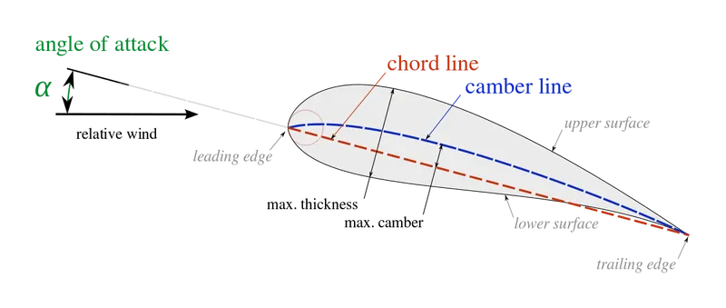
Source: https://en.wikipedia.org/wiki/Airfoil
The leading edge is the point at the front of the airfoil that has maximum curvature (minimum radius).
The trailing edge is defined similarly as the point of maximum curvature at the rear of the airfoil.
The chord line is the straight line connecting leading and trailing edges. The chord length, or simply chord, is the length of the chord line. That is the reference dimension of the airfoil section.
The mean camber line or mean line is the locus of points midway between the upper and lower surfaces. Its shape depends on the thickness distribution along the chord.
The camber is the maximum distance between the mean camber line and the chord line, measured normal to the chord line.
The thickness is the distance between the upper and lower surfaces also measured normal to the chord line. For example, an airfoil of the NACA 4-digit series such as the NACA 2415 (to be read as 2 – 4 – 15) describes an airfoil with a camber of 0.02 chord located at 0.40 chord, with 0.15 chord of maximum thickness.
The upper and lower surfaces are also known as suction and pressure surfaces respectively. Upper surface is generally associated with higher velocity and lower static pressure, while lower surface has a comparatively higher static pressure than the suction surface. The pressure gradient between these two surfaces contributes to the lift force generated for a given airfoil.
NACA0017 Airfoil:
The profile of NACA0017 airfoil is shown below:
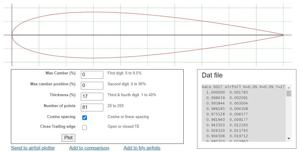
Source: http://airfoiltools.com/airfoil/naca4digit
The specifications can be described as an airfoil whose camber is 0% of the chord, the maximum camber is located at 0% of the chord and thickness is 0.17 or 17% of the chord.
Procedure for modeling:
A new Part file was opened in SolidWorks, with MKS units and then the data of airfoil was used to generate a curve using Insert --> Curves --> Curve through XYZ points.
On the dialog box that appears, the text file containing Airfoil data was browsed, selected and opened, after which the data can be seen in a table form.
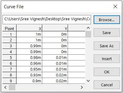
After clicking on Ok, the Airfoil was generated.
Using Convert entities, the airfoil curve was converted to a sketch and then using Line command, a line was drawn to make the Airfoil as a closed contour, as shown below:
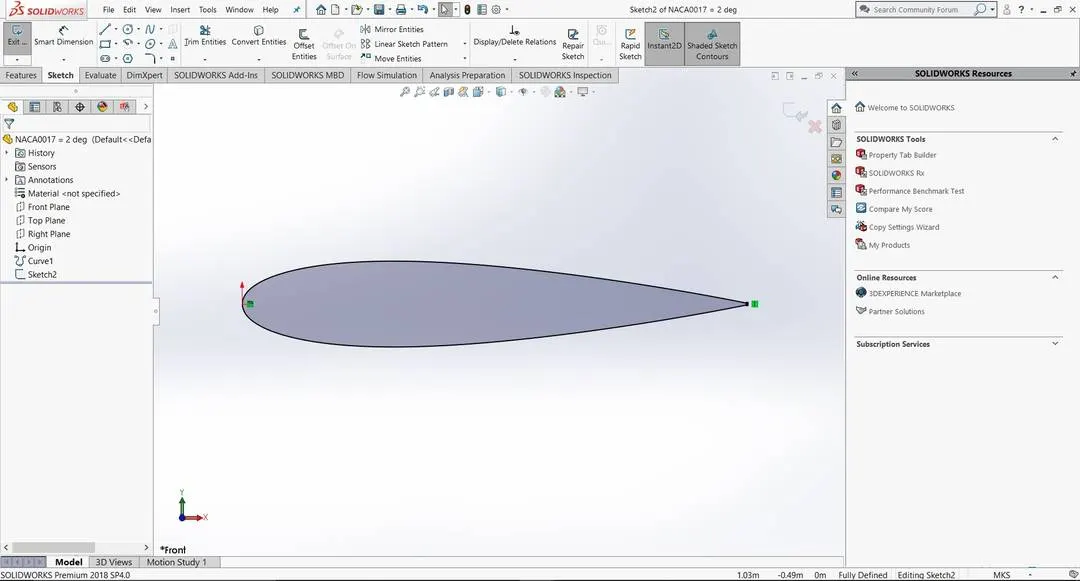
The angle of attack was specified using Rotate entities command and choosing the appropriate angles, depending on the different cases. An image showing the rotated profile for one of the cases, where angle of attack is 2 degrees is shown below:
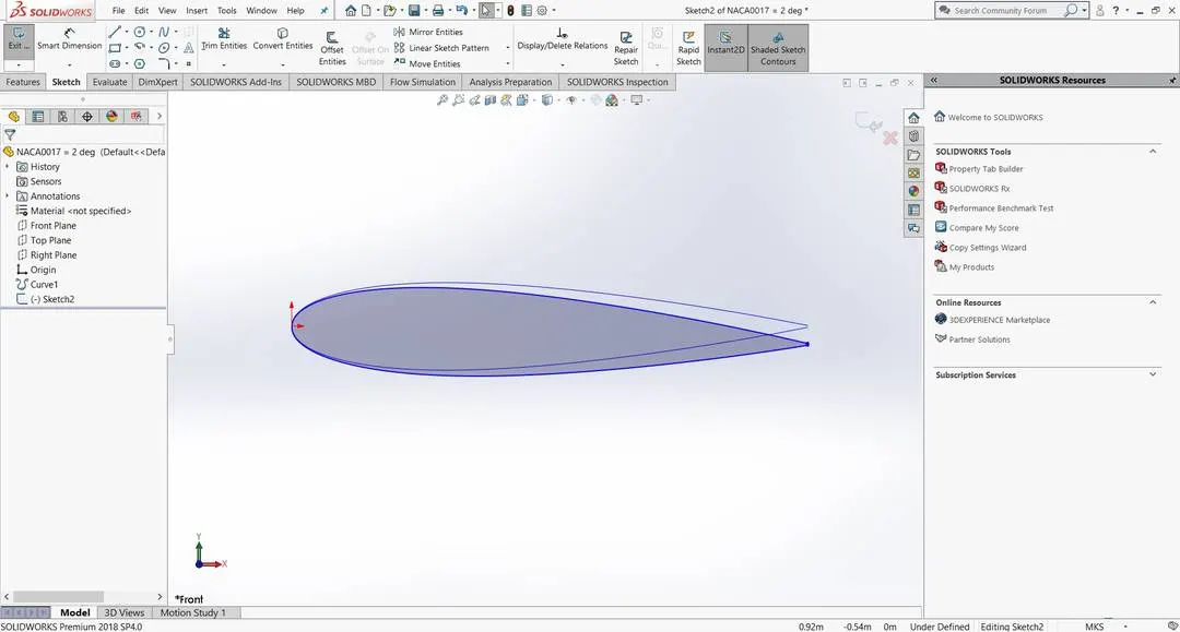
Using Extrude command, the sketch was extruded for 0.5m to get a 3D geometry of the Airfoil. Since it was a 2D simulation, the length of extrusion is however, not a consideration.
Case setup:
Once the Airfoil was modeled, Flow simulation was enabled using SolidWorks Add-Ins.
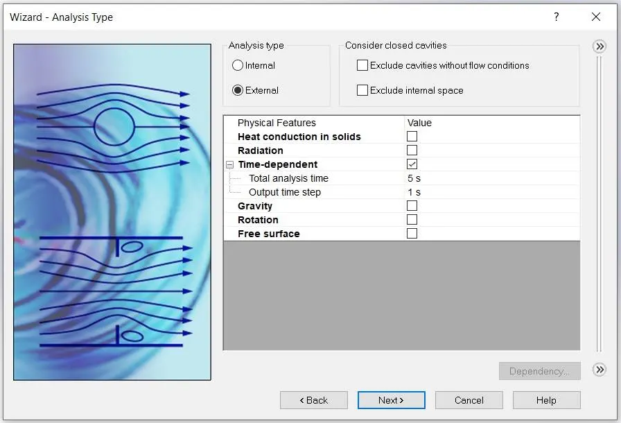
In the Wizard, a suitable name was given for the study and then External analysis was selected. A Time-dependent study was chosen, where the Total analysis time was taken as 5s and Output time step as 1s, so as to get 5 outputs.
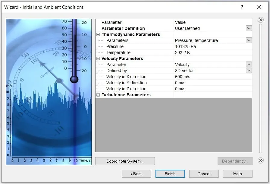
Air(Gases) was selected as the working fluid and Velocity was chosen as 600m/s. All the other conditions were left as default.
The Computational domain definition was edited as 2D simulation and along X and Y directions. Then, the distance between end point of the Airfoil and right side boundary is extended in such a way that it is 10-15 times the Chord length and distance between front end of the Airfoil and left side boundary as 5 times the Chord length. Along Y axis, the domain length was considered to be 5-7 times the Chord length.
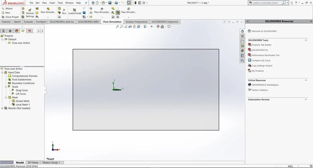
Then Goals were added so as to visualize Drag Force and Lift Force and Cut plots along XY planes for Pressure and Velocity were defined.
The whole geometry was meshed and the surface on the top was refined further using Local mesh settings.
The simulation was Run and Output plots and Goal plots were visualized.
Results:
(a) `0^0` angle of attack:
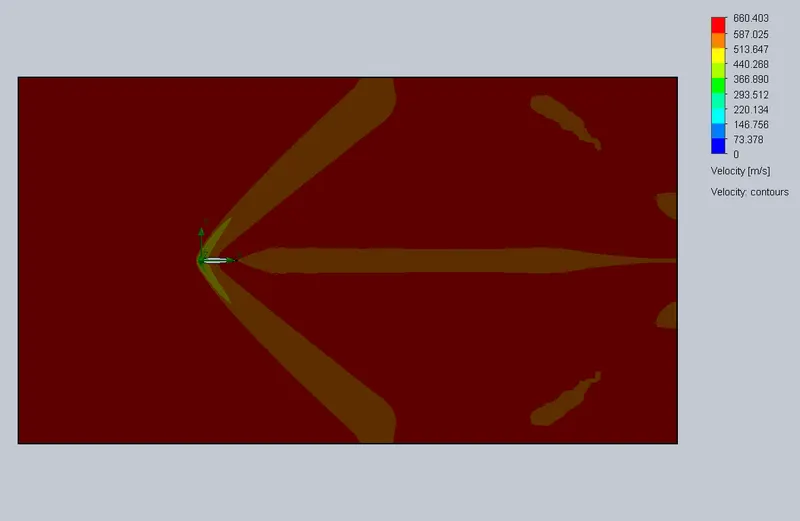
Velocity cut plot:
Pressure cut plot:
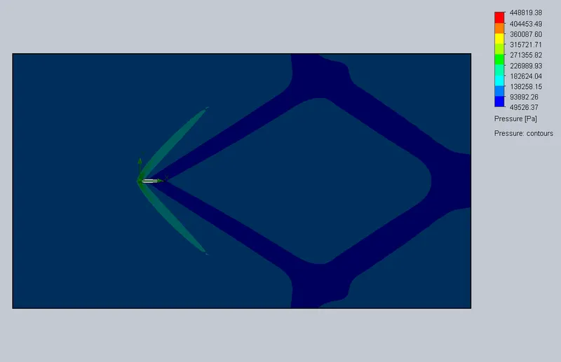
Velocity and Pressure profiles are symmetrical when the Angle of attack is 0 degrees.
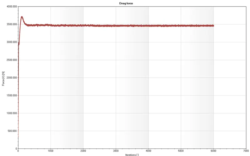
Drag Force:
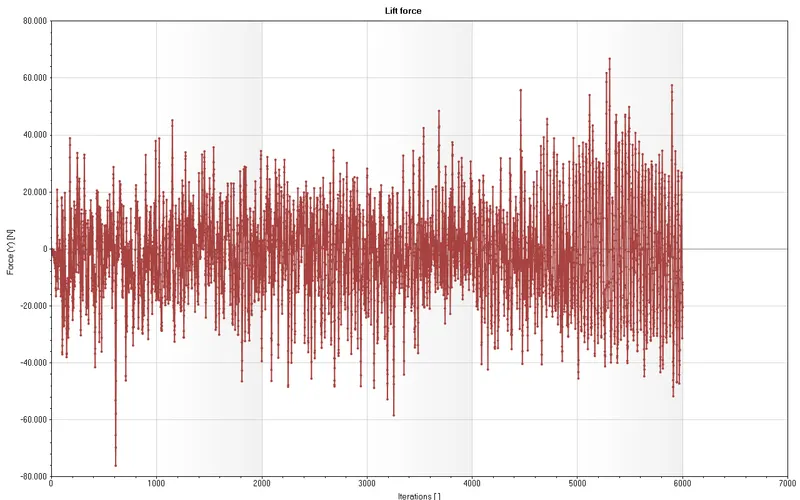
Lift Force:
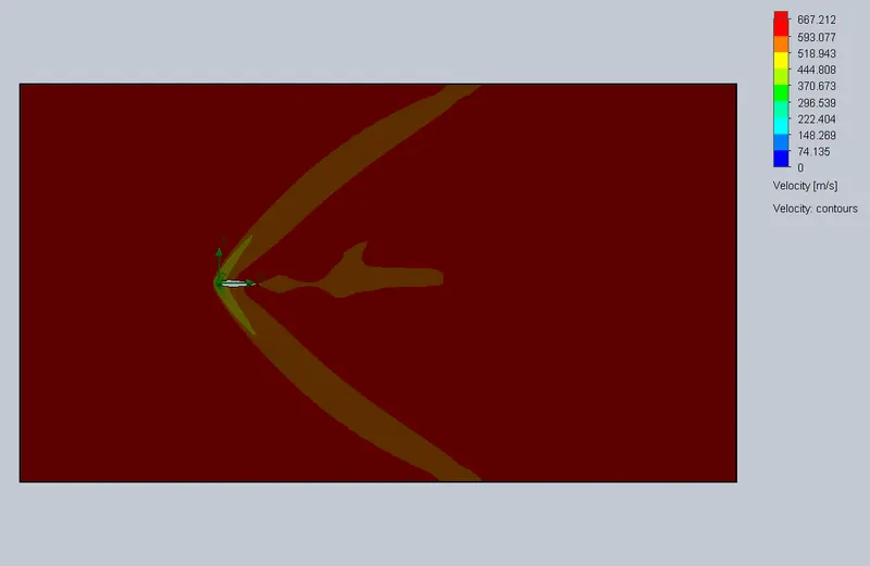
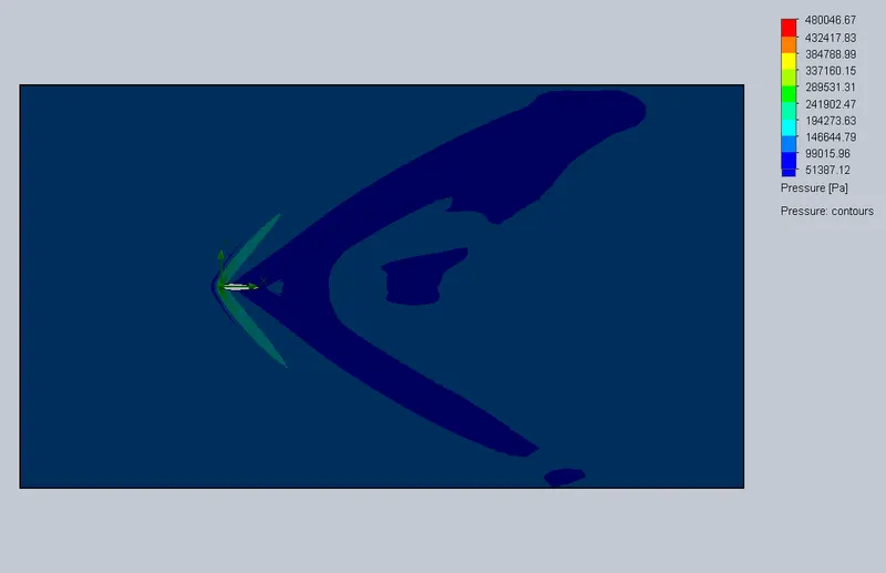
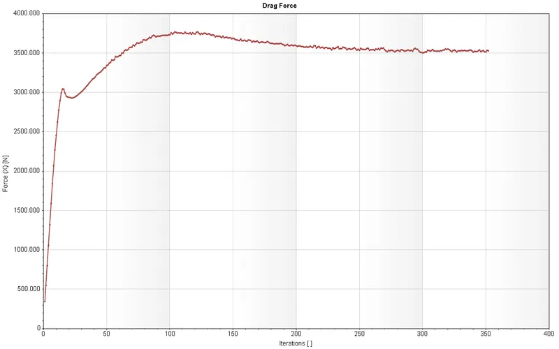
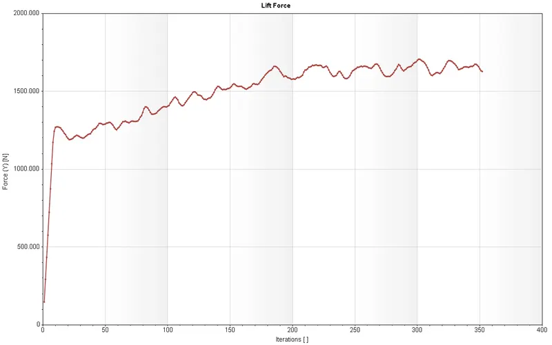
(b) `2^0` angle of attack:
Velocity cut plot:
Pressure cut plot:
Drag Force:
Lift Force:
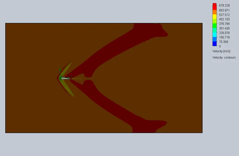
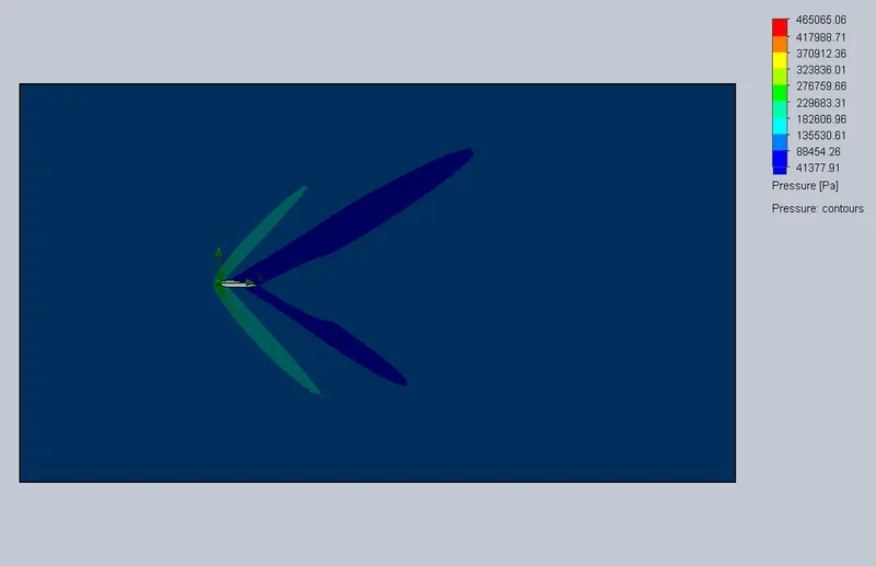
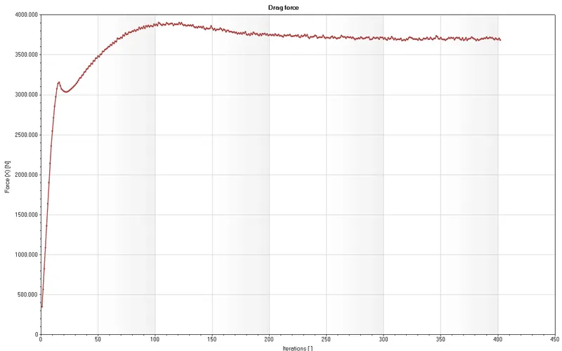
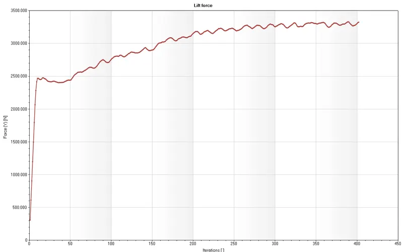
(c) `4^0` angle of attack:
Velocity cut plot:
Pressure cut plot:
Drag Force:
Lift Force:
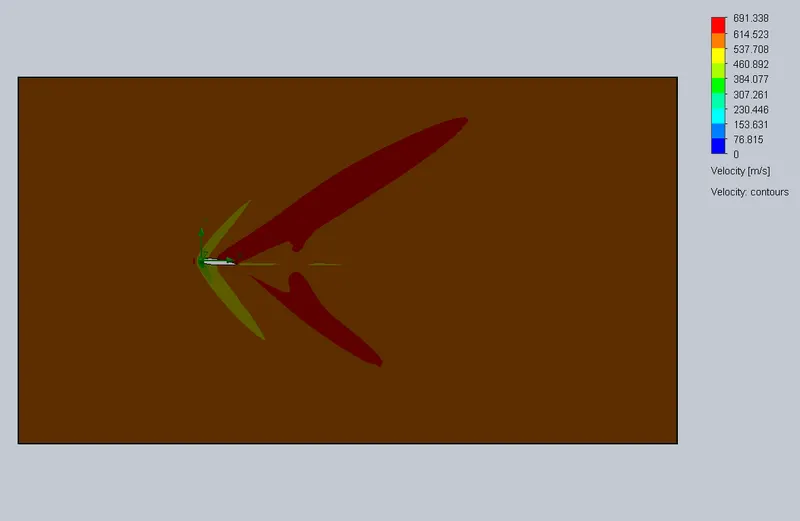
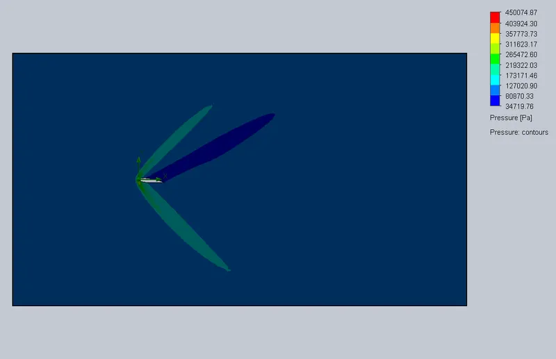
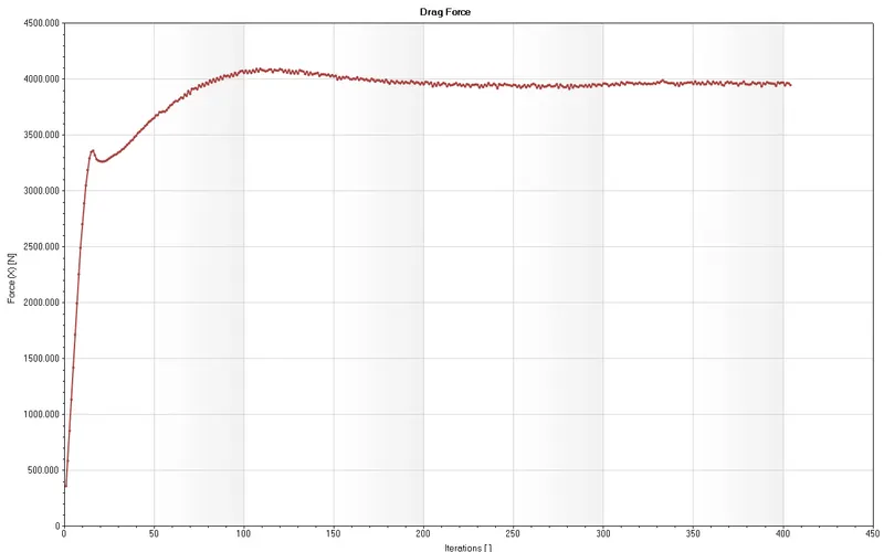
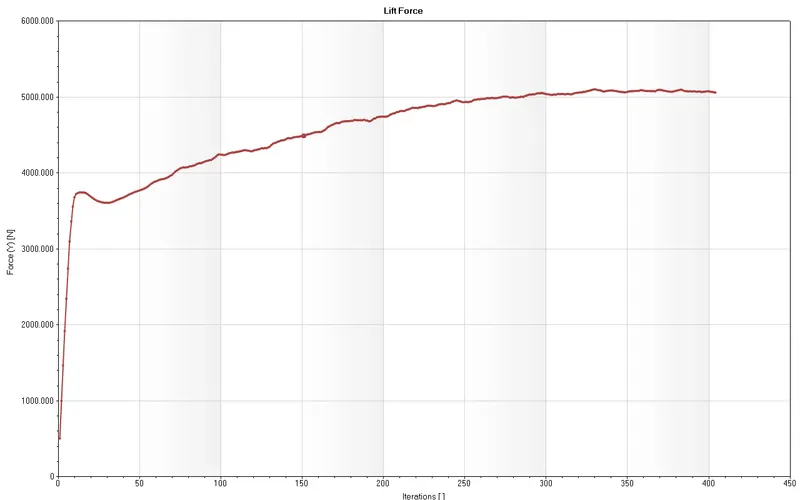
(d) `6^0` angle of attack:
Velocity cut plot:
Pressure cut plot:
Drag Force:
Lift Force:
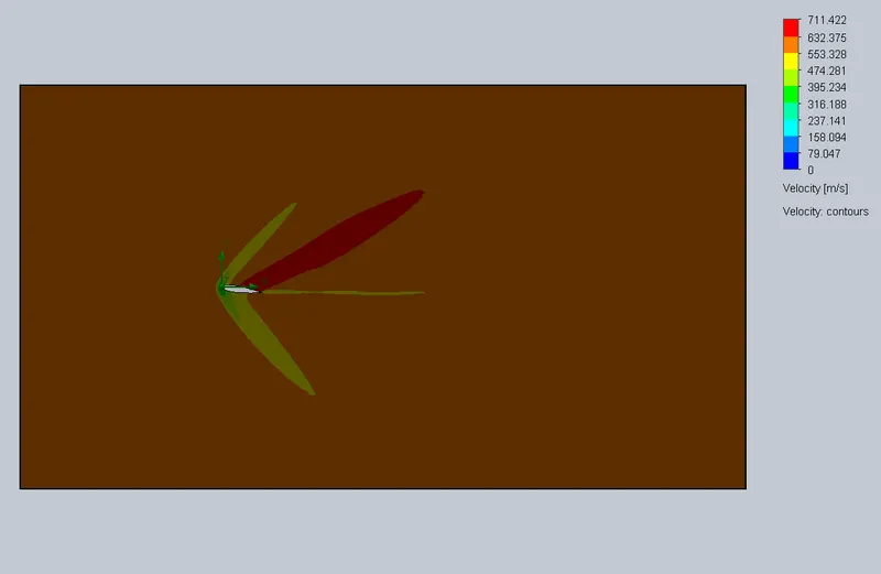
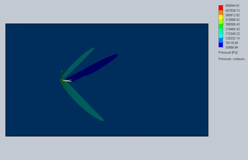
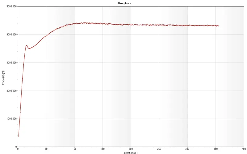
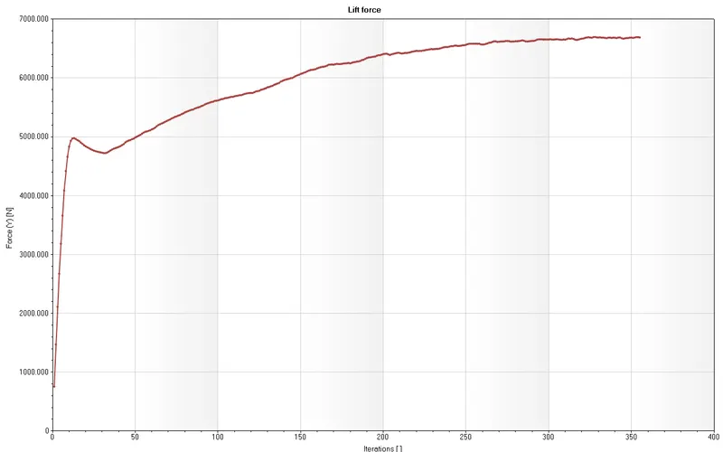
(e) `8^0` angle of attack:
Velocity cut plot:
Pressure cut plot:
Drag Force:
Lift Force:
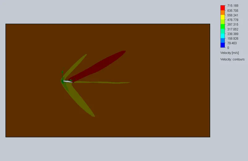
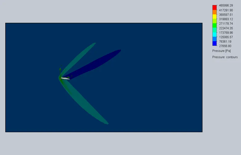
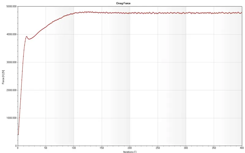
(f) `10^0` angle of attack:
Velocity cut plot:
Pressure cut plot:
Drag Force:
Lift Force:
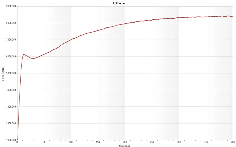
In all the above plots, the Drag force is the force that acts along the X-direction and Lift force acts vertically upwards along the Y-direction. The drag and lift forces increase in each case when the angle of attack increases.
(g) Comparison of Drag and Lift forces based on Angle of attack:
|
S.No |
Angle of attack (deg) |
Averaged Drag Force (N) |
Averaged Lift Force (N) |
|
1 |
0 |
3463.622923 |
-6.818227237 |
|
2 |
2 |
3528.869499 |
1654.168836 |
|
3 |
4 |
3702.635298 |
3295.182192 |
|
4 |
6 |
3964.090671 |
5079.612557 |
|
5 |
8 |
4325.909958 |
6667.878951 |
|
6 |
10 |
4769.060741 |
8381.871078 |
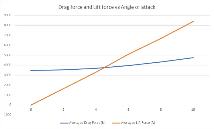
Drag and lift forces increase as the angle of attack increases. Below 4 degrees, drag force is greater than lift force which indicates the unsuitable conditions for flying. Above 4 degrees, the lift force tends to increase greater than drag force and at a value of around 5 degrees and above, the lift force increases considerably higher than drag force, which indicates suitable conditions for flying.
Observations:
As the angle of attack is varied the lift and drag change very rapidly due to changes in pressure distribution over the airfoil.
At lower angles of attack, the lift arises from the difference between the pressure reduction on the upper and lower surfaces. At higher angles of attack, the lift is partly due to pressure reduction on the upper surface and partly due to pressure increase on the lower surface.
The airfoil will be able to fly when the angle of attack is 4 degrees to 10 degrees, based on this study. It is because, only for these values of angles of attack, the lift force is greater than the drag force.
At angles of attack above 5 degrees, there is a drastic change in the value of Drag force because of the increased frontal area compared to the cases below 5 degrees.
Consequent to changes in pressure distribution due to change of angle of attack, there will be a movement of the center of pressure. As the angle of attack increases, the center of pressure tends to move towards the leading edge of the airfoil until the stalling angle is reached.
Conclusion:
Flow over NACA0017 airfoil was simulated and the drag and lift forces for various angles of attack were compared. The results were visualized in the form of plots and attached in report along with observations and explanations.
References: