Simulation of flow over a cylinder
Aim:
- To run a baseline simulation for flow over a cylinder and calculate the Reynolds number.
- To increase the Reynolds number by a factor of 20%, 40%, and 100% then run the transient flow simulation.
Introduction:
(a) Steady state flow and Transient flow:
A flow that is not a function of time is called steady flow. Steady-state flow refers to the condition where the fluid properties at a point in the system do not change over time. Time dependent flow is known as transient or unsteady flow. Whether a particular flow is steady or unsteady, can depend on the chosen frame of reference.
Steady flows are often more tractable than otherwise similar unsteady flows. The governing equations of a steady problem have one dimension fewer (time) than the governing equations of the same problem without taking advantage of the steadiness of the flow field.
(b) Reynolds Number:
The Reynolds number (Re) helps predict flow patterns in different fluid flow situations and it is the ratio of inertial force to the viscous force.
It is mathematically defined as:
`Re = (rho u l)/mu = (u l)/v`
where:
ρ is the density of the fluid (kg/m3)
u is the flow speed (m/s)
L is a characteristic linear dimension (m) (In our case, it is the diameter of the cylinder)
μ is the dynamic viscosity of the fluid (Pa·s or N·s/m2 or kg/(m·s))
ν is the kinematic viscosity of the fluid (m2/s)
At low values of Re, the flow is laminar. When Re exceeds a certain threshold, semi-developed turbulence occurs in the flow; this regime is usually referred to as “transition regime” and occurs for a certain range of the Reynolds number. Finally, over a certain value of Re, the flow becomes fully turbulent. The mean value of Re in the transition regime is usually named “Critical Reynolds number” and it is considered the threshold between the laminar and the turbulent flow.
Procedure for Modeling:
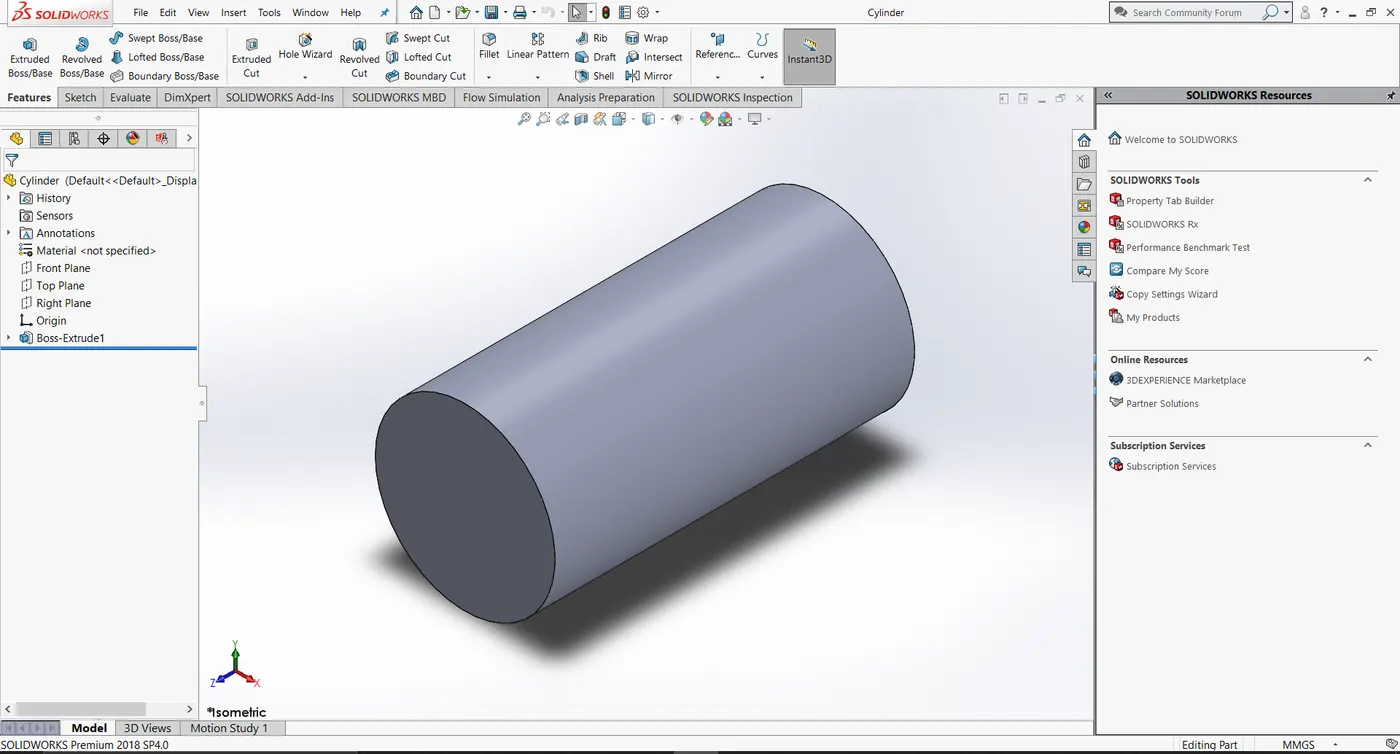
A cylinder was modeled with the following dimensions:
Diameter (D) = 50mm
Height(H) = 100mm
First, a circle was drawn on one of the planes for 50mm diameter using Sketch tools and then using Extruded Boss/Base command, it was extruded to 100mm to form a cylinder.
Calculation of parameters:
The fluid was taken as Air(Gases)
Properties of Air are:
Density `rho` = `1.225 (kg)/(m^3)`
Dynamic Viscosity `mu` = `1.81 * 10^-5 (N-s)/(m^2)`
Calculation of Reynolds number:
`Re = (rho v D)/mu`
For base line simulation, Total analysis time was 0.1 seconds and output time step was 0.01 seconds. Flow velocity v was taken as 10m/s. Thus,
`Re = ((1.225)*10*(0.05))/(1.81*10^-5) = 33839.78`
Therefore, for the other three cases, Reynolds number is calculated as:
In Case 1, for 20% increase,
`Re = 33839.78 + (33839.78*0.2) = 40607.73`
Similarly in Case 2, for 40% increase `Re = 47375.69`
And in Case 3, for 100% increase, `Re = 67679.56`
Calculation of Velocity:
Since the value of Reynolds number for the three cases is known, the velocities can be calculated by using the formula of Re itself.
`implies v = (Re*mu)/(rho*D)`
Hence, for Case 1, when `Re = 40607.73`, the velocity `v = (40607.73*1.81*10^-5)/(1.225*0.05)= 12m/s`
Similarly, for Case 2, when `Re = 47375.69`, the velocity `v = 14m/s`
And for Case 3, when `Re = 67679.56`, the velocity `v = 20m/s`
Calculation of End time:
To compute the end time and time step for the rest of the simulations, we need to know two parameters namely, Length of the computational domain and the Flow through time.
Length of the domain = `0.275+0.175 = 0.450 m`
This length remains the same for all the simulations since the geometry is the same.
Flow through time is defined as the time taken by the fluid to flow from inlet to outlet. It is calculated as Length of the Domain/Inlet velocity of the fluid.
The end time is taken as 2*Flow through time.
Hence, for Case 1,
Flow through time = `0.450/12 = 0.0375 s`
End time = `2*0.0375 = 0.075s`
Similarly, for Case 2,
Flow through time is `0.032s` and End time is `0.064s`
And for Case 3,
Flow through time is `0.0225s` and End time is `0.045s`
Case Setup and procedure:
Flow simulation was enabled from SolidWorks Add-Ins.
For the entire simulation, External Analysis type was selected from the Flow simulation Wizard and also, Time-dependent study was enabled, where there are options to enter Total analysis time and output time step. Time-dependent study is used to simulate Transient flow.
Once the parameters were calculated, the simulation data were set accordingly for each case using the Wizard.
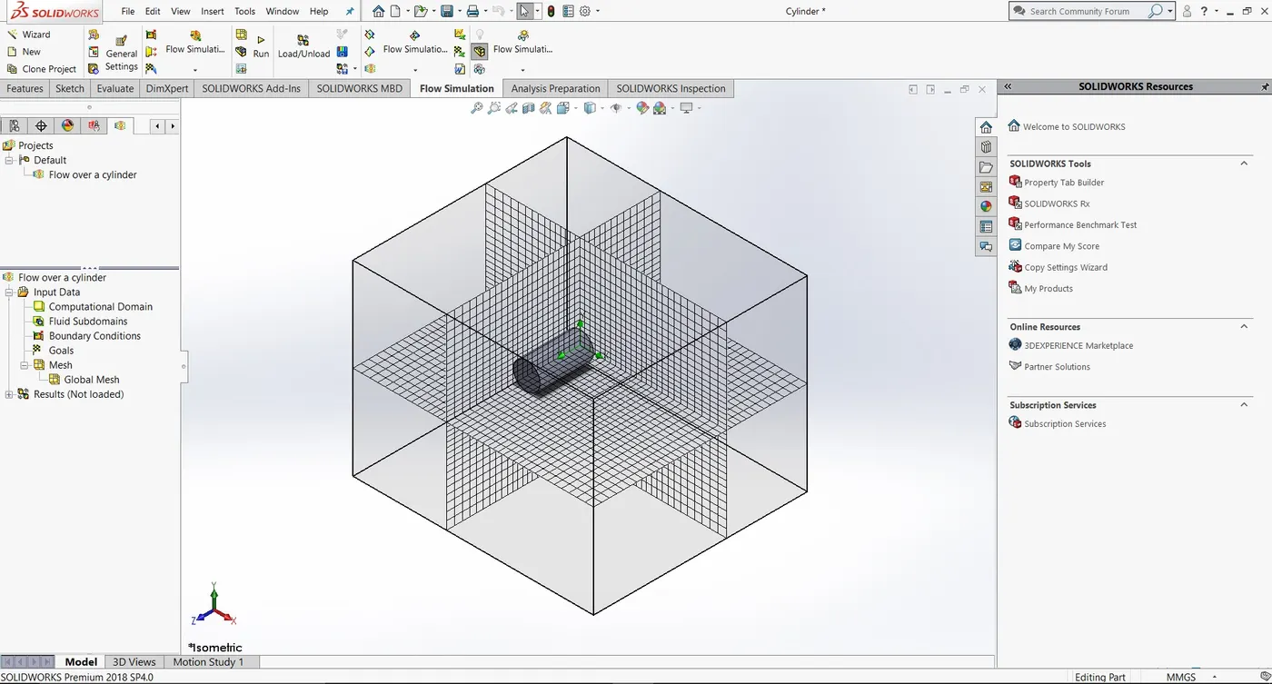
A finer Mesh was chosen under Global Mesh for all the three cases in order to obtain close to accurate results.
The computational domain along with the mesh is shown in the image below:
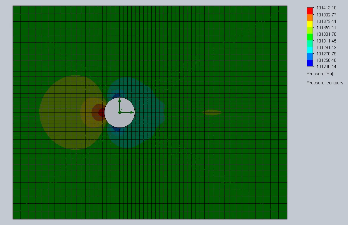
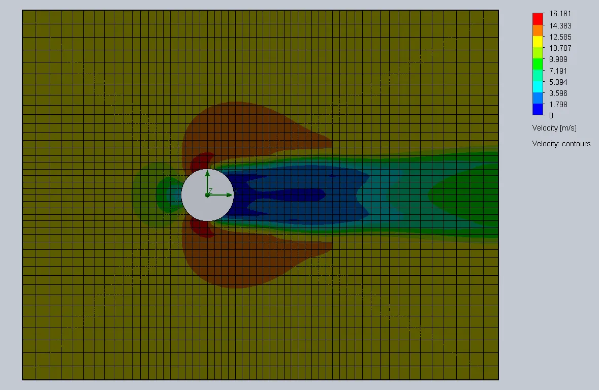
From the results, Cut plots were chosen for Pressure and Velocity for all the three simulations.
The simulation was then Run and the plots were visualized.
A new animation was created from Results menu for both Pressure and Velocity for all the three cases using Animation Wizard.
Results:
(a) Case 1 (20% increase in Re):
Pressure cut plot:
Velocity Cut plot:
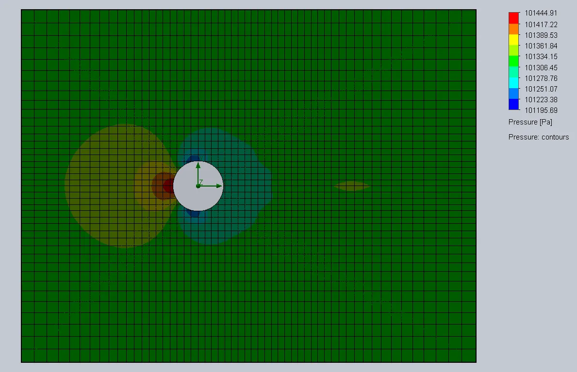
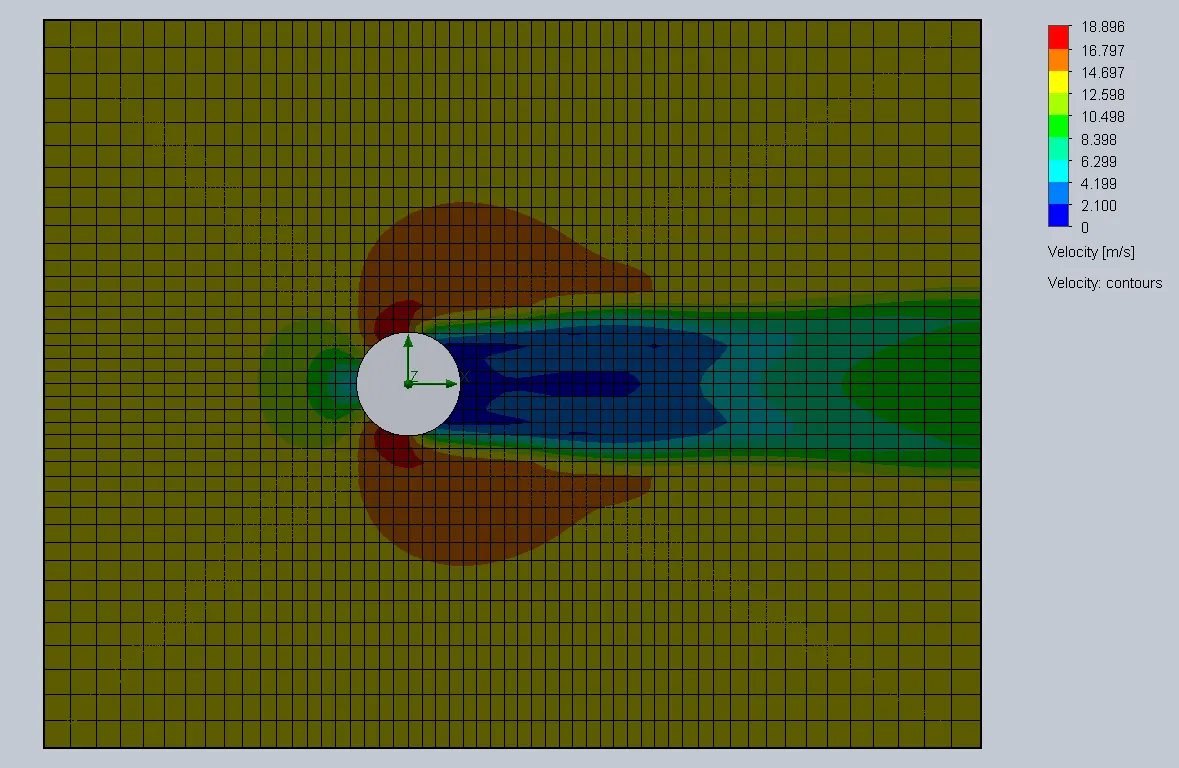
(b) Case 2 (40% increase in Re):
Pressure cut plot:
Velocity Cut plot:
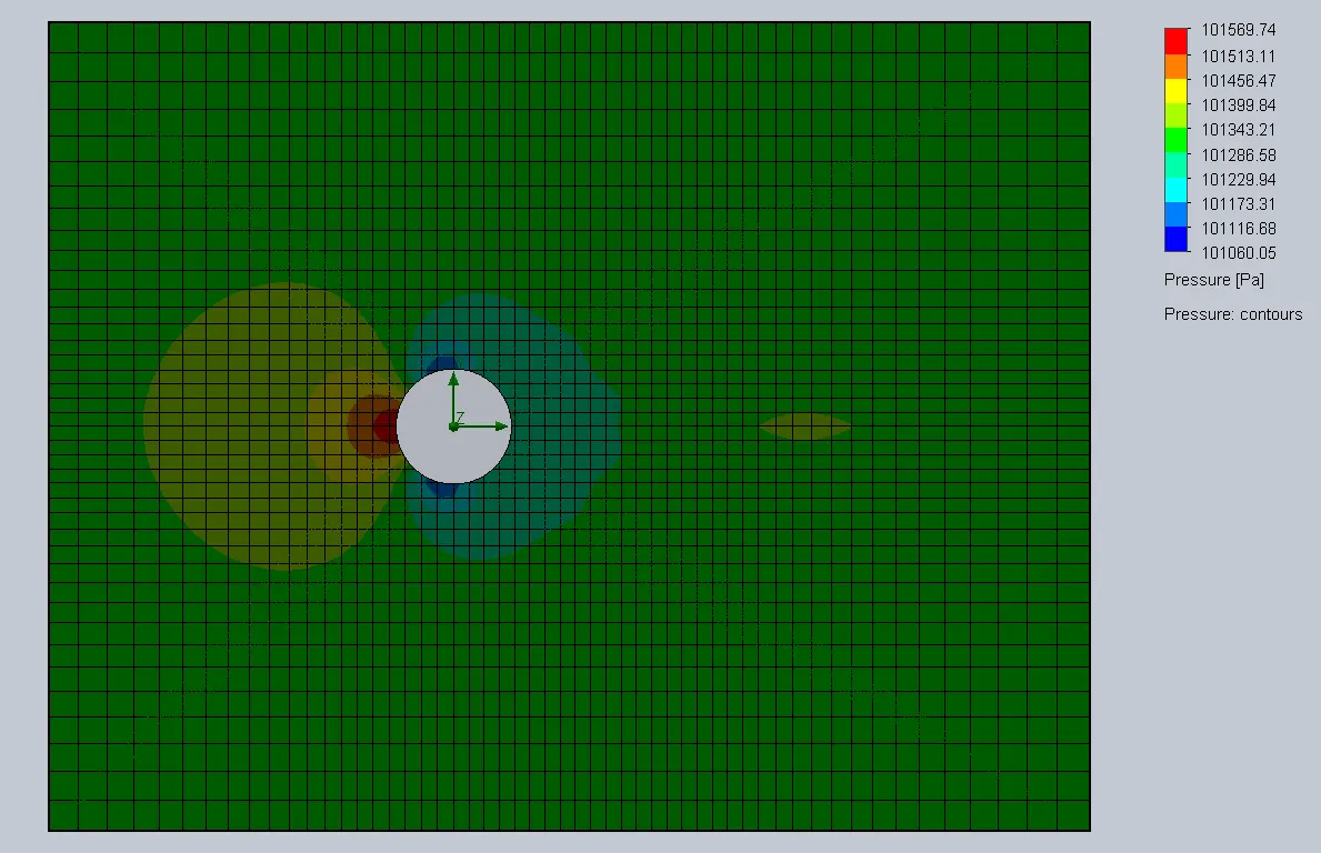
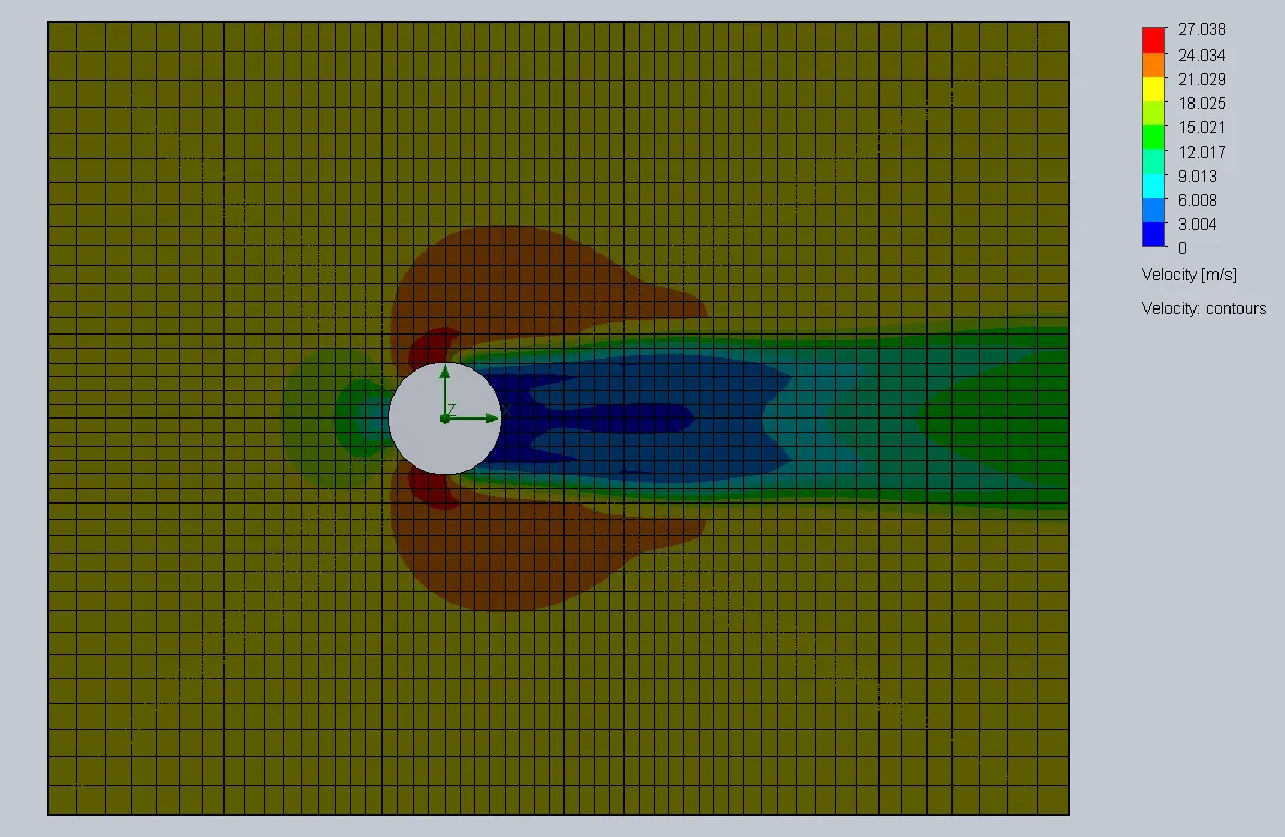
(c) Case 3 (100% increase in Re):
Pressure cut plot:
Velocity Cut plot:
Animations for all the three cases is found in the Google Drive link below:
https://drive.google.com/drive/folders/1Fh4XIMc9O4ylKDzxPDbilRNaDKQvNWb9?usp=sharing
Observations:
As the Reynolds number increases, velocity also increases and so the flow through time decreases. When the Reynolds number and velocity increase, the flow changes from laminar to turbulent.
Mathematically, when Re increases by 20%, velocity also increases by 20% and also for 40% and 100% increase in Re, velocity increases by 40% and 100% respectively. Thus, Reynolds number and Velocity are directly proportional.
There is a pressure difference between the front and back of the cylinder. Since the pressure at the front side is greater, the velocity is lower on the front side and due to low pressure on the back of the cylinder, velocity is greater on the back side.
According to the results from the pressure plot, it is clear that the pressure is the highest on the frontal area of the cylinder.
More accurate results can be obtained with a fine meshing than a coarse meshing.
Conclusion:
Flow over a cylinder was simulated for the given conditions and the results were visualized in the form of cut plots and detailed explanation about my observations were given. Also, animations of the simulation for all the three cases were provided in the report.
References: