Second Order ODE solving for Simulate the movement of simple pendulum

Aim- A program to simulate the transient behaviour of a simple pendulum and to create an animation of its motion

Software- MatLab

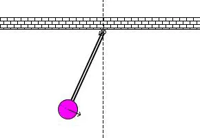
Sub Objectives:-

• Write a program to solve the ODE
• Plot the displacement v/s time & velocity v/s time graphs
• Create an animation of the motion of the pendulum

Theory-

In Mathematics, an ordinary differential equation(ODE) is a differential equation containing one or more functions of one independent variable and the derivatives of those functions. The term ordinary is used in contrast with the term partial differential equation which may be with respect to more than one independent variable.

Here, we are using the ODE that represents the motion of a simple pendulum with damping. The general equation for this is:

We are going to use this 2nd order ODE equation to find out the velocity and position of the pendulum ball with respect to time.

b = damping coefficient

m = mass of the body

g = gravitational force

L = length of the pendulum

solving the ode-

Whenever we are given a second-order differential equation we break it into two first-order equations and solve them, now the equation can be solved as follows-

So here we need to solve for theta1 and theta2 which are the displacements and velocities of the bob respectively. Let's write a code for it.

Inputs-

L=1 metre,

m=1 kg,

b=0.05.

g=9.81 m/s2.

% Initial consitions given are- initial displacement =0;initial velocity =5.

Now we create a column vector theta_0 to store these both values%

theta_0=[0;5];

% Given we have a time span of 0 t0 20 sec ,considser we take 500 values between them.

t_span=linspace(0,10,500);

now we need to write code to solve the two single order equations .we create another function file to import the function.

we create the function solution which takes the values t,theta,b,m,l,g as inputs to solve our ode's.

function [dtheta_dt]= solution(t,theta,b,m,l,g)

we already know that if theta is differentiated once we get displacement and if it is differentiated twice we get velocity. so we call the values from the initial array theta_0 and store them in theta1, theta2

theta1=theta_0(1)
theta2=theta_0(2)

Now we enter the two differential equations we obtained after splitting them and store the output in another array

dtheta1_dt=theta2;
dtheta2_dt=-(b/m)*theta2- (g/l)*sin(theta1);
[dtheta_dt]=[dtheta1_dt;dtheta2_dt];

After the function file is created we use a ode solver command in the original file to solve the ode.

The command we use is ode45

[t,results]=ode45(@(t,theta)solution(t,theta,b,m,l,g),t_span,theta_0);

here @(t,theta) is to specify that they are variables.

solution(t,theta,b,m,l,g) is a function that is called from file solution.m with inputs of t,theta,b,m,l,g.

t_span is the time integration array.

theta_0 is the initial conditions array.

We store all the output in an array [t, results], where results are a two-row vector containing both theta1(displacement),theta2(velocity).

In order to plot the moment of the pendulum, we need to know the positions of its ends at each time interval. So we take one end(point1) of the pendulum as fixed and other ends (point2) to be varying. If we join the two ends by a line we get a figure having a line inclined at an angle theta with the axis.

If we resolve it into components we get x= l*sin(theta)

y=-l*cos(theta)[along -ve y axis]

So now the coordinates of point two is (l*sin(theta),-l*cos(theta)) .

So now we need to run a for loop for varying values of theta so that we can find the various positions of point2. We join the two points with a line.

Also, we need a bob at its end i.e at point 2, so we create a marker using marker command and give its size and line width. To get the picture that is shown in the introduction part we need several plot commands according to the introduction.

for i=1:length(results)
theta=results(i);
x1=l*sin(theta);
y1=-l*cos(theta);

plot([-0.5 0.5],[0 0],'linewidth',5,'color','b')

hold on

plot([0 0],[-1.5 1.5],'-.','color','r')
plot([0,-0.05],'o','markersize',9,'color','b')
plot([0 x1],[-0.05 y1],'linewidth',8,'color','y')

plot(x1,y1,'o','markersize',20,'linewidth',20,'color','r')
grid on

plot(x1,y1,'-')
hold off

axis([-1.5 1.5 -1.5 1])
M(ct)=getframe(gcf);
ct=ct+1;

end

Now our graph is plotted in order to get a movie out of it we need to capture the frames and store it in an array M by using a command called getframe(gcf).

We use a variable ct to give a position to a particular frame and increment it each time a frame is captured.

Then we create a video file and then write the video into that file and close it.

movie(M)
v=VideoWriter('ode_main.avi','uncompressed avi')
open(v)
writeVideo(v,M)
close(v)

function code-

filename- ode_func

function [dtheta_dt]= ode_func(t,theta,b,g,l,m)
  
  theta1= theta(1)
  theta2= theta(2)
  dtheta1_dt= theta2;
  dtheta2_dt= -(b/m)*theta2 - (g/l)*sin(theta1)
  dtheta_dt= [dtheta1_dt; dtheta2_dt];
end

Main Program Function-

filename- ode_main

%solving a ode
close all
clear all
clc
%INPUTS
b=0.05;
l=1;
g=9.81;
m=1;
%initial conditions
theta_0=[0;5];
%time span
t_span=linspace(0,10,500);
%solve
[t,results]=ode45(@(t,theta)ode_func(t,theta,b,g,m,l),t_span,theta_0);
ct=1;
for i=1:length(results)
    theta=results(i);
    x1=l*sin(theta);
    y1=-l*cos(theta);
    
    plot([-0.5 0.5],[0 0],'linewidth',5,'color','b')
     
    hold on
   
    plot([0 0],[-1.5 1.5],'-.','color','r')
    plot([0,-0.05],'o','markersize',9,'color','b')
    plot([0 x1],[-0.05 y1],'linewidth',8,'color','y')
    
    plot(x1,y1,'o','markersize',20,'linewidth',20,'color','r') 
    grid on 
    
    plot(x1,y1,'-')
    hold off
     
    axis([-1.5 1.5 -1.5 1])
   M(ct)=getframe(gcf);
    ct=ct+1;
end
movie(M)
v=VideoWriter('ode_main.avi','uncompressed avi')
open(v)
writeVideo(v,M)
close(v)

Output-

The differential equation is solved and the displacement, velocity values at given time intervals are found out so that the movement of the pendulum can be tracked.