MatLab code to solve otto cycle,generate p-v graph and calculate thermal efficiency

Objective- Write a code that can solve an Otto cycle, generate p-v plot and calculate thermal efficiency of the engine

Software Used- MatLab

Description-

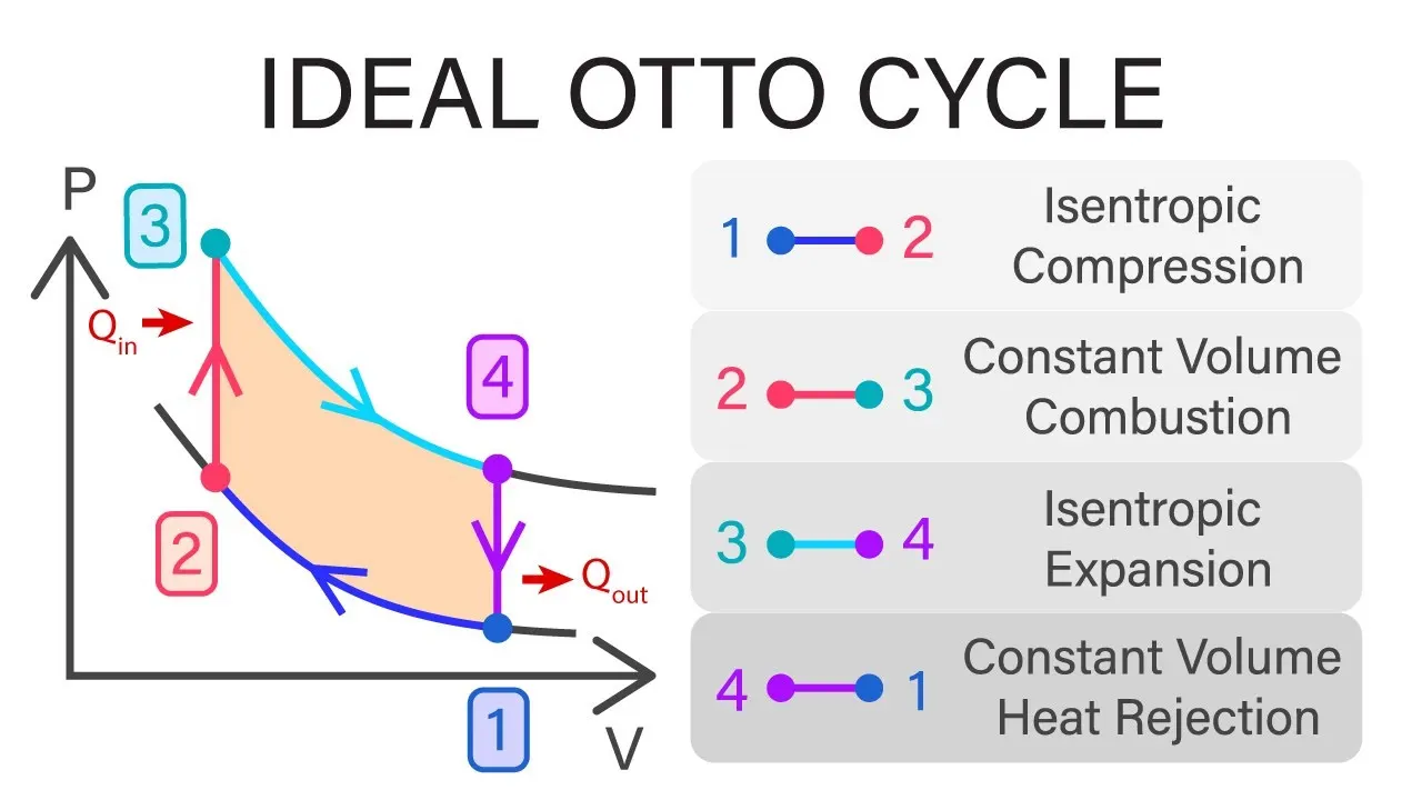
process 1-2 -isentropic compression

P*V^gamma = constant

T*V^(gamma-1) = constant

process 2-3 -the constant volume of heat addition

process 2-4 -Isentropic expansion

process 4-1 -the constant volume of heat rejection

Thermal efficiency = 1-1/cr^(gamma-1)

we need to calculate pressure, volume and the temperature at each point 1,2,3,4

Calculation of swept and clearance volume (using engine parameters)

v_swept= (pi/4)*bore^2*stroke;

v_clearance = v_swept/(cr-1);

v1=v_swept+v_clearance; (total volume of cylinder)

v2=v_clearance; (volume after compression)

Engine parameters-

bore=0.1;

stroke=0.1;

con_rod=0.15;

cr=12; %(compression ratio)

gamma=1.4;

Input parameters-

p1=101325; %in pascals = 1 atm

t1=500;

t3=2300;

v3=v2;

calculation of variables at all 4 points-

point 1-

p1=101325;

t1=500;

v1=v_swept+v_clearance;

point 2-

v2=v_clearance;

p2=p1*cr^gamma;

t2= (p2*v2*t1)/(p1*v1);

const_c=p1*v1^gamma;

point 3-

t3=2300;

v3=v2;

p3= p2*t3/t2;

point 4-

v4 = v1;

p4=p3/cr^gamma;

Program-

close all
clear all
clc
%inputs
bore=0.1;
stroke=0.1;
con_rod=0.15;
cr=12;
gamma=1.4;
%caluclation of swept volume and clearnace volume
v_swept= (pi/4)*bore^2*stroke;
v_clearance = v_swept/(cr-1);
%state variables at 1(p in pascals and t in k)
p1=101325;
t1=500;
v1=v_swept+v_clearance;
%state variables at 2
v2=v_clearance;
p2=p1*cr^gamma;
t2= (p2*v2*t1)/(p1*v1);

%state variables at 3 assume temperature after compression =
t3=2300;
v3=v2;
p3= p2*t3/t2;
%state variables at 4
v4 = v1;
p4=p3/cr^gamma;
efficiency = 1-1/( cr^(gamma-1))

hold on
plot(v1,p1,'*','color','r')
plot(v2,p2,'*','color','r')
plot(v3,p3,'*','color','r')
plot(v4,p4,'*','color','r')
plot([v1,v2,v3,v4],[p1,p2,p3,p4])
xlabel('volume')
ylabel('pressure')

Output-

we can see in the output that point 1 and 2 are joined linearly bur we know that they vary according to the equation. it is also same in process 3 and 4 so now during the expansion and

compression process, the dependency of pressure and volume is not linear.

so we need an equation to find the compressed and expanded volumes and corresponding compressed and expansion pressure

we have a relation

v/v_c=1+.5(cr-1)[R+1-cosd(theta)-(R^2-(sind^2(theta)^.5)]

where theta is the crank angle

r=connecting rod length/a;

a=stroke/2;

we vary the theta from start crank angle to the end crank angle using linspace command

theta=linspace(0,180,180);

Program-

clear all
close all
clc
bore=0.1
stroke=0.1
cond_rod=0.15
cr=12
a=stroke/2
R=cond_rod/a
v_s=pi/4*bore^2*stroke;
v_c=v_s/(cr-1);
%v/v_c=1+.5(cr-1)[R+1-cosd(theta)-(R^2-(sind^2(theta)^.5)]
theta=linspace(0,180,180);
term1=0.5*(cr-1);
term2=R+1- cosd(theta);
term3=(R^2-sind(theta).^2).^0.5;
v=(1+term1*(term2 - term3)).*v_c;
plot(theta,v)
xlim([0 180])

output-

when theta = linspace(0,180,180) when theta = linspace(0,720,720)

theta - (x-axis), volume - (y-axis) theta - (x-axis), volume - (y-axis)

main program-

During compression, crank rotates 180 to 360

v_compression=engine_kinematics(bore,stroke,con_rod,180,360);

const_c=p1*v1^gamma;

p_compression= const_c./(v_compression).^gamma

during expansion crank rotates from 360 to 540 degrees

v_expansion=engine_kinematics(bore,stroke,con_rod,360,540);

cont_c=p3*v3^gamma;

p_expansion = cont_c./(v_expansion).^gamma;

efficiency = 1- 1/(cr^(gamma-1))

now we plot the graph

plot(v_compression,p_compression,'color','b','linewidth',2)

plot(v_expansion,p_expansion,'color','b','linewidth',2)

main program-

close all
clear all
clc
%inputs
bore=0.1;
stroke=0.1;
con_rod=0.15;
cr=12;
gamma=1.4;
%caluclation of swept volume and clearnace volume
v_swept= (pi/4)*bore^2*stroke;
v_clearance = v_swept/(cr-1);
%state variables at 1(p in pascals and t in k)
p1=101325;
t1=500;
v1=v_swept+v_clearance;
%state variables at 2
v2=v_clearance;
p2=p1*cr^gamma;
t2= (p2*v2*t1)/(p1*v1);
v_compression=engine_kinematics(bore,stroke,con_rod,180,360);
const_c=p1*v1^gamma;
p_compression= const_c./(v_compression).^gamma

%state variables at 3 assume temperature after compression =
t3=2300;
v3=v2;
p3= p2*t3/t2;
%state variables at 4
v4 = v1;
p4=p3/cr^gamma;

v_expansion=engine_kinematics(bore,stroke,con_rod,360,540);
cont_c=p3*v3^gamma;
p_expansion = cont_c./(v_expansion).^gamma;
efficiency = 1- 1/(cr^(gamma-1))

hold on
plot(v1,p1,'*','color','r')
plot(v2,p2,'*','color','r')
plot(v_compression,p_compression,'color','b','linewidth',2)
plot(v3,p3,'*','color','r')
line(v2,v3,'color','g')
plot(v_expansion,p_expansion,'color','b','linewidth',2)
plot(v4,p4,'*','color','r')
plot([v2,v3],[p2,p3],'color','b','linewidth',2)
plot([v4,v1],[p4,p1],'color','b','linewidth',2)
xlabel('volume')
ylabel('pressure')

require output-