Road Classification and The PSD Profile (Week 10_b challenge)
MATLAB CODE
clear all;
clc;
%% INPUT
% Road data
% freq in cycle/ft
% amplitude in ft^2/(rad/ft)
freq = [0.004 0.190
0.190
0.205
0.210
0.215
0.220
0.235
0.250
0.255
0.275
0.280
0.283
0.285
0.300
0.310
0.320
0.330
0.340
0.350
0.353
0.355
0.360
0.370
0.375
0.380
0.385
0.395
0.410
0.420
0.425
0.430
0.435
0.438
0.440
0.460
0.463
0.465
0.480
0.485
0.486
0.490
0.500
0.510
0.540
0.545
0.560
0.005
0.006
0.007
0.008
0.009
0.010
0.012
0.017
0.020
0.024
0.028
0.043
0.055
0.063
0.068
0.071
0.080
0.083
0.089
0.090
0.098
0.105
0.115
0.128
0.135
0.145
0.150
0.154
0.160
0.165
0.166
0.167
0.175
0.180
0.185
0.188
0.565
0.575
0.585
0.590
0.595
0.610
0.620
0.630
0.650
0.655
0.660
0.670
0.680
0.685
0.686
0.690
0.695
0.696
0.700
0.705
0.710
0.715
0.720
0.725
0.730
0.740
0.750
0.765
0.780
0.790
0.810
0.815
0.820
0.830
0.850
0.855
0.860
0.870
0.880
0.885
0.890
0.900];
amplitude = [0.006759586
0.013802191
0.012220044
0.012805345
0.010055096
0.008674203
0.009906454
0.013565614
0.038077859
0.039514035
0.039376401
0.029351388
0.011087978
0.007155759
0.004009582
0.005053475
0.005426501
0.002758627
0.003146703
0.004278752
0.003605323
0.001118033
0.004605136
0.001110531
0.001926103
0.000599825
0.000790703
0.00082178
0.001138063
0.000449034
0.000344602
0.000439721
0.000485891
0.000661237
0.000247849
0.000282707
0.000336575
0.000260436
0.000338
0.000334243
0.000339473
0.000258116
0.000296182
0.000286092
0.000377324
0.000235117
0.000158941
0.000351811
0.000475459
0.000269363
0.00013499
0.000410917
0.000243289
0.000183098
0.000224051
0.000614261
0.000355537
0.000239772
0.000288619
0.000268181
0.00037814
0.000279647
0.000210043
0.000159755
0.000224234
9.50236E-05
0.000197943
0.000138383
0.000143463
0.00012055
0.000161674
9.97741E-05
8.9633E-05
0.000122986
0.000172037
0.000102941
0.00012442
9.02789E-05
0.000143594
6.29552E-05
9.28956E-05
0.000144869
0.000181894
0.000119478
0.000128017
0.000154808
0.000109269
0.000107822
9.00107E-05
0.000123476
8.48896E-05
0.000116729
0.000156981
0.000189126
0.000140362
0.000287068
0.000162162
0.000229266
0.000138612
7.98678E-05
0.000149275
7.12492E-05
0.00022861
8.03851E-05
0.000140036
5.64396E-05
9.09341E-05
0.000118502
7.68087E-05
7.41522E-05
0.000101869
4.47478E-05
0.000103792
0.000164574
9.03105E-05
9.00065E-05
0.000148517
0.000169078
8.09882E-05
9.06266E-05
9.01182E-05
6.61969E-05
0.000101917
5.92651E-05
6.81185E-05
];
% three frequencies
omega(1)=0.01;
omega(2)=1/(2*pi())
omega(3)=10;
%% GENERATE ROAD ROUGHNESS CLASS LINES
s_a(2)=8*10^-6;
s_b(2)=32*10^-6;
s_c(2)=128*10^-6;
s_d(2)=512*10^-6;
s_e(2)=2048*10^-6;
s_f(2)=8192*10^-6;
s_g(2)=32768*10^-6;
s_h(2)=90000*10^-6;
s_a(1)=s_a(2)*(omega(1)/omega(2))^-2;
s_a(3)=s_a(2)*(omega(3)/omega(2))^-1.5;
s_b(1)=s_b(2)*(omega(1)/omega(2))^-2;
s_b(3)=s_b(2)*(omega(3)/omega(2))^-1.5;
s_c(1)=s_c(2)*(omega(1)/omega(2))^-2;
s_c(3)=s_c(2)*(omega(3)/omega(2))^-1.5;
s_d(1)=s_d(2)*(omega(1)/omega(2))^-2;
s_d(3)=s_d(2)*(omega(3)/omega(2))^-1.5;
s_e(1)=s_e(2)*(omega(1)/omega(2))^-2;
s_e(3)=s_e(2)*(omega(3)/omega(2))^-1.5;
s_f(1)=s_f(2)*(omega(1)/omega(2))^-2;
s_f(3)=s_f(2)*(omega(3)/omega(2))^-1.5;
s_g(1)=s_g(2)*(omega(1)/omega(2))^-2;
s_g(3)=s_g(2)*(omega(3)/omega(2))^-1.5;
s_h(1)=s_h(2)*(omega(1)/omega(2))^-2;
s_h(3)=s_h(2)*(omega(3)/omega(2))^-1.5;
loglog(omega,s_a,'linewidth',3);
hold on;
loglog(omega,s_b,'linewidth',3);
hold on;
loglog(omega,s_c,'linewidth',3);
hold on;
loglog(omega,s_d,'linewidth',3);
hold on;
loglog(omega,s_e,'linewidth',3);
hold on;
loglog(omega,s_f,'linewidth',3);
hold on;
loglog(omega,s_g,'linewidth',3);
hold on;
loglog(omega,s_h,'linewidth',3);
set(gca,'fontsize',15);
xlabel('spatialfrequency (cycle/m)','fontsize',18);
ylabel('powerspectraldensity m^2/(cycle/m)','fontsize',18);
title('road classification by iso');
legend('A','B','C','D','E','F','G','H');
hold off;
%% PSD PROFILE PLOTTING
loglog(freq,amplitude);
xlabel('spatialfrequency (cycle/m)','fontsize',18);
ylabel('powerspectraldensity m^2/(cycle/m)','fontsize',18);
title(' PSD PLOT');
Explanation of the code for Road classification
Considering three frequencies omega1, omega2, omega3, where omega2 is the break point, we find the road roughness class lines using the below equation,
`S(omega) = S(omega_o)*(omega/omega_o)^-2` for `omega_0 < omega_n`
`S(omega) = S(omega_o)*(omega/omega_o)^-1.5` for `omega_0 > omega_n`
`S(omega_o)` is the road roughness`
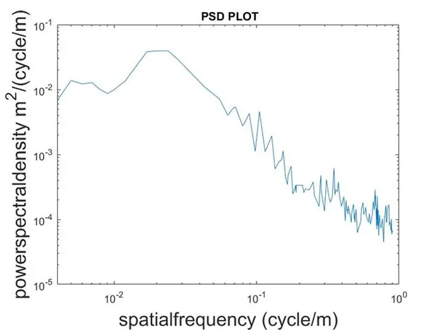
Explanation of the code for PSD profile
Given: The amplitude and the frequency is given.
It can be inserted in Matlab by simply copying and pasting the given data.
log log plot takes the log on both x and y axes .
Therefore loglog(freq,amplitude) gves the desired PSD profile.
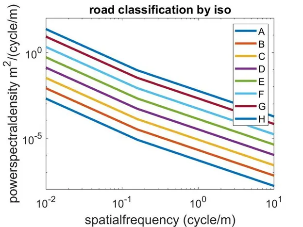
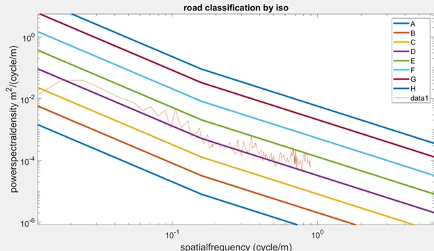
Road profile obtained is CLASS D: because the PSD curve fits the curve D, which has a degree of roughness of max `2048*10^-6` m2/cycle/m. It is a poor Road.
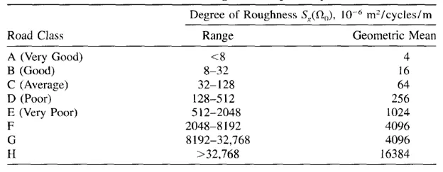
It can be identified from the above data.
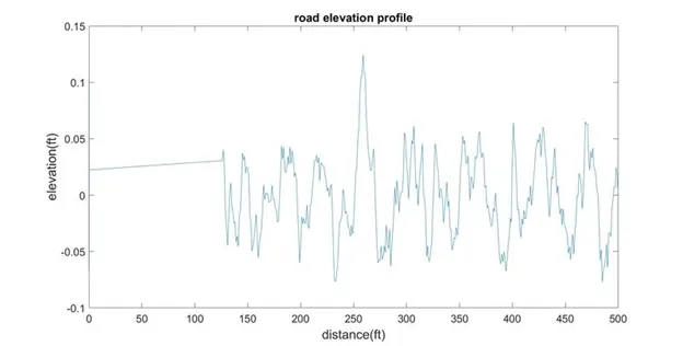
ROAD ELEVATION PROFILE (PLOT)
%% generate space domain profile from roughness PSD
delta_sigma(1) = freq(2) - freq(1);
delta_sigma(125) = freq(125) - freq(124);
for j=2:124;
delta_sigma(j) = (freq(j+1) - freq(j-1))/2;
end
for j=1:500;
x(j) = j;
total(j) = 0;
for i=1:125
x(i) = sqrt(amplitude(i)*2*delta_sigma(i))
total(j) = total(j) + x(i)*sin(freq(i)*x(j)*2*pi());
end
end
figure(3);
plot(x,total);
set(gca,'fontsize',15);
xlabel('distance(ft)','fontsize',18);
ylabel('elevation(ft)','fontsize',18);
title('road elevation profile');