Reaction Mechanism Reduction

AIM

The aim of this project is to analyse the reduction in reaction mechanism of GRI Mech 3.0

OBJECIVES

• Program to run a reference Ignition delay and Max temperature Analysis for the unreduced mechanism for a set of state values
• Sensitivity analysis with respect to temperature must be run on all the reactions in the mechanism and must sort the reactions from the most sensitive to least sensitive.
• These sorted reactions should be added to a new mechanism file/object one by one starting from a fixed minimum number of reactions.
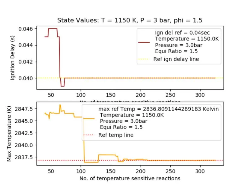
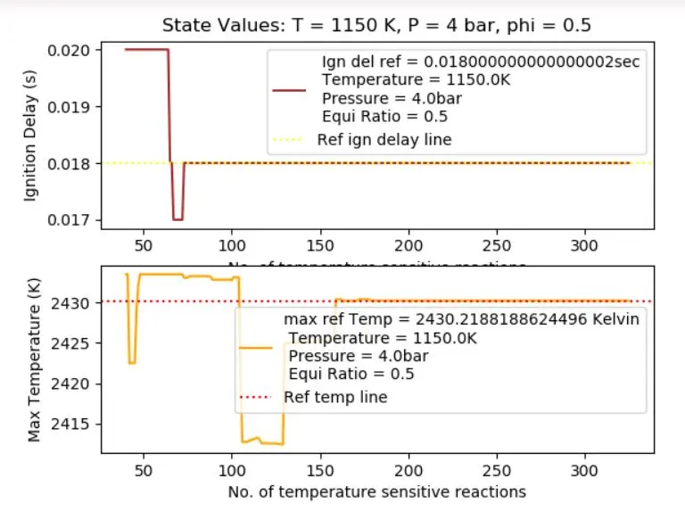
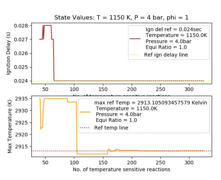
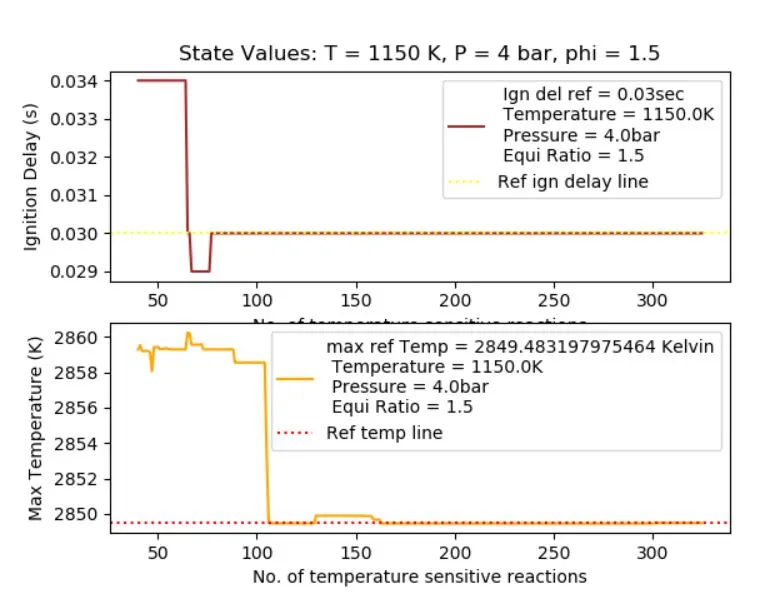
• Graph for plotting the reduced mechanism's ignition delay and max temperature while having the reference ignition delay and Temperature as a label for reference

REACTION REDUCTION MECHANISM

Increases in both chemical kinetics knowledge and the capacity of computers have led to the availability of very large detailed kinetic mechanisms for many problems. These mechanisms may contain up to several thousand species and several ten thousand reaction steps. For computational reasons, however, large mechanisms still cannot be used in spatially 2D or 3D computational fluid dynamics simulations, where the applied mechanism typically requires less than 100 species. Also, within such large mechanisms, the key processes can be masked by the presence of many reaction steps of only marginal importance. A first step to reducing the size of a kinetic mechanism is to identify species and reaction steps which do not need to be included in order to accurately predict the key target outputs of the model. Such methods lead to so-called “skeletal” schemes. Many different methods for the identification of redundant species and reaction steps within a mechanism, including those based on sensitivity and Jacobian analyses, the comparison of reaction rates, trial and error and calculated entropy production. Another family of methods for the development of skeletal schemes is based on the investigation of reaction graphs. We discuss here the directed relation graph (DRG) method and its derivatives, and the path flux analysis (PFA) method. Mechanism reduction may be also based on optimisation methods which minimise an objective function related to the simulation error between the full and reduced models, subject to a set of constraints (e.g. numbers of species required). Integer programming and genetic algorithm-based methods have been used for such an optimisation. From these skeletal schemes, subsequent reductions can be achieved via either species or reaction lumping. Chemical and mathematical approaches to lumping are discussed with applications in combustion, atmospheric and biological systems. Reduction methods based on timescale separation are then introduced starting with the classic quasi-steady-state approximation (QSSA). Computational singular perturbation (CSP) methods are then described as a means of informing the derivation of analytically reduced models. Further efficiency gains can also be obtained by using a numerical approximation of a function in place of more traditional descriptions of chemical source terms within simulation models. The generation of such numerical reduced models can be based on the original differential equations and the thermodynamics of the problem or deduced from the simulation results. Using any of these methods, the applied function has to meet special requirements, such as the need to be evaluated quickly and to provide an accurate approximation. We discuss a series of approaches, tabulation methods, artificial neural networks (ANNs) and various
types of polynomials, that all have been tested and applied within the context of kinetic modelling.

One of the barriers to using complex kinetic mechanisms within larger models of reactive flows is the computational time required to solve the resulting rate equations. If the full comprehensive mechanism is used, then this may lead to compromises being required in modelling other aspects of the flow. Using a coarser model grid resolution is often a compromise that has to be made within computational fluid dynamics (CFD) codes. The more species that are included within the chemical model, the lower the grid resolution that can be afforded on a given hardware architecture. Simplifications of turbulent mixing processes may also have to be made. For example, it is unlikely that highly detailed chemistry could be afforded within a 3D direct numerical simulation of a problem where attempts are made to resolve all important timescales of turbulent
mixing. It follows that when trying to couple a chemical kinetic model with a complex physical model, the important dynamics of the chemical system should be represented as efficiently as possible, i.e. with the lowest number of variables possible.

MECHANISM REDUCTION PARAMETERS FILE

Temperature	950 1050 1150
Pressure	300000 400000 500000
Phi		0.5 1 1.5	

PROGRAM FOR REDUCTION IN REACTION MECHANISM

import os 
import cantera as ct 
import matplotlib.pyplot as plt 
import numpy as np 

# Extracting mech_reduction date from 'mech_reduction_file' using user-defined class 'FileReader' 
class FileReader: 
	def __init__(self, filename):
		self.filename = filename 
		self.mech_reduction_dict = {} 

	def validate_file(self): 
		return os.path.isfile(self.filename) 

	def read(self): 
		if self.validate_file(): 
			for line in open(self.filename, 'r'): 
				self.mech_reduction_dict[line.split()[0]] = line.split()[1:] 
			
		else: 
			print('No file under such name') 
a = FileReader('mech_reduction.txt') 
a.read() 
T1 = [float(x) for x in a.mech_reduction_dict['Temperature']] 
P1 = [float(x) for x in a.mech_reduction_dict['Pressure']] 
equivalence_ratio = [float(x) for x in a.mech_reduction_dict['Phi']] 
size = 40 
S = [] 
pw_max = [] 
ind1 = [] 
n = 0 
t_end = 5 
dt = 0.001 
tol_Tmax = 0.05 
tol_ignd = 0.05 
gas = ct.Solution('gri30.xml') 
S_max = [0]*gas.n_reactions 
spec = ct.Species.listFromFile('gri30.xml')
K7 = [] 
ignd_a1 = [] 
Tmax_b1 = [] 
size_of_mech = [] 
case = 1 
for T in T1: 
	for P in P1: 
		for phi in equivalence_ratio: 
			gas.TP = T, P 
			gas.set_equivalence_ratio(phi, 'CH4', 'O2:1, N2:3.76') 
			r = ct.IdealGasReactor(gas) 
			sim = ct.ReactorNet([r]) 
			
			for i in range(0, gas.n_reactions): 
				r.add_sensitivity_reaction(i) 
			sim.rtol = 1e-6 
			sim.atol = 1e-15 
			sim.rtol_sensitivity = 1e-6 
			sim.atol_sensitivity = 1e-6 
			
			for t in np.arange(0, t_end+dt, dt): 
				sim.advance(t) 
				
				for i in range(0, gas.n_reactions): 
					S = sim.sensitivity(2, i) 
					if np.abs(S) > np.abs(S_max[i]): 
						S_max[i] = np.abs(S) 
			for i in range(0, gas.n_reactions): 
				pw_max.append([]) 
				pw_max[i].append(np.abs(S_max[i])) 
				pw_max[i].append(i) 
			# sorting p4_max array in decreasing order of sensitivity 
			S_sorted = sorted(pw_max, key = lambda x: x[0], reverse = True) 
			# appending the sorted order of reaction indices to indl 
			for i in range(0, gas.n_reactions): 
				
				ind1.append([]) 
				ind1[i].append(S_sorted[i][1]) 
			
			pw_max.clear() 
			n = n + 1 

R_set = set() 
R_ordered = [] 
for i in range(0, gas.n_reactions): 
	for j in range(0, n): 
		if ind1[i][j] not in R_set: 
			R_ordered.append(ind1[i][j]) 
			R_set.add(ind1[i][1]) 
print(R_ordered, n) 
# Determining the size of the reduced mechanism 
for T in T1: 
	for P in P1: 
		for phi in equivalence_ratio: 
		# computing reference ign_delay and T_max for each state 
			T_ign = T + 400 # K 
			gas.TP = T, P 
			gas.set_equivalence_ratio(phi, 'CH4', 'O2:1, N2:3.76') 
			r = ct.IdealGasReactor(gas) 
			sim = ct.ReactorNet([r]) 
			Tmax_r = 0 
			c1 = True 
			for t in np.arange(0, t_end+dt, dt): 
			
				sim.advance(t)

				if (T_ign < gas.T and c1 is True):
					ignd_r = t
					c1 = False

				if (Tmax_r < gas.T):
					Tmax_r = gas.T

			error_Tmax = 0
			error_ignd = 0
			i = 0
			c3 = True

			for i in range(0, gas.n_reactions): 
				K7.append(gas.reaction(R_ordered[i])) 
				gas1 = ct.Solution(thermo = 'IdealGas', kinetics = 'GasKinetics', species = spec, reactions = K7) 
				gas1.TP = T, P 
				gas1.set_equivalence_ratio(phi, 'CH4', 'O2:1, N2:3.76') 
				r1 = ct.IdealGasReactor(gas1) 
				sim1 = ct.ReactorNet([r1]) 
				T_max = 0 
				c2 = True 
			
				for t in np.arange(0, t+dt, dt): 
					sim1.advance(t) 
					if ( T_ign < gas1.T and c2 is True): 
						ign_delay = t 
						c2 = False 
				
					if ( T_max < gas1.T): 
						T_max = gas1.T 
				# reaction index increment 
				i = i + 1 
			# finding exceptions until the no. of reactions increases to a suitable number 
				try : 
					if (i >= size) : 
						ignd_a1.append(ign_delay) 
						Tmax_b1.append(T_max) 
						size_of_mech.append(i) 
				# calculating the error 
					error_Tmax = np.abs(((Tmax_r - T_max)/Tmax_r)*100) 
					error_ignd = np.abs(((ignd_r - ign_delay)/ignd_r)*100) 

# printing the values of phi, temperature etc. when the tolerance value is satisfied 
					if (error_Tmax < tol_Tmax and error_ignd < tol_ignd and c3 is True): 
						print('T = %g, P = %g, phi = %g, Tmax_r = %g, ignd_r = %g, T_max = %g, ign_delay = %g, T_max_error = %g, Ign_delay_error = %g, red_size_mech = %g' %(T, P, phi, Tmax_r, ignd_r, T_max, ign_delay, error_Tmax, error_ignd, i)) 
						c3 = False 

				except NameError: 
					pass 
			plt.subplot(211)
			plt.title('State Values: T = %g K, P = %g bar, phi = %g' %(T, P/100000, phi)) 
			plt.plot(size_of_mech, ignd_a1,color = 'brown',label = 'Ign del ref = ' +str(ignd_r) + 'sec' + 'n Temperature = ' + str(T) + 'K' + 'n Pressure =' + str(P/100000)) + 'bar' + 'n Equi Ratio =' + str(phi)
			plt.axhline(y = ignd_r, color = 'yellow', linestyle = ':', label = 'Ref ign delay line') 
			plt.xlabel('No. of temperature sensitive reactions') 
			plt.ylabel('Ignition Delay (s)') 
			plt.legend(loc = 'best') 
			plt.subplot(212) 
			plt.plot(size_of_mech, Tmax_b1, color = 'orange',label = 'Max ref Temp = ' +str(T_max) + 'Kelvin' + 'n Temperature = ' + str(T) + 'K' + 'n Pressure =' + str(P/100000)) + 'bar' + 'n Equi Ratio =' + str(phi)) 
			plt.xlabel('No. of temperature sensitive reactions') 
			plt.ylabel('Max Temperature (K)') 
			plt.legend(loc = 'best')
			plt.tight_layout()
			plt.show()

			K7.clear()
			ignd_a1.clear()
			T_max.claer()
			size_of_mech.clear()
			case +=1

PLOTS FOR THE CODE

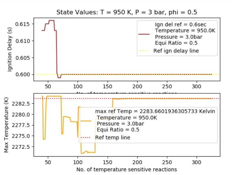
Case 1

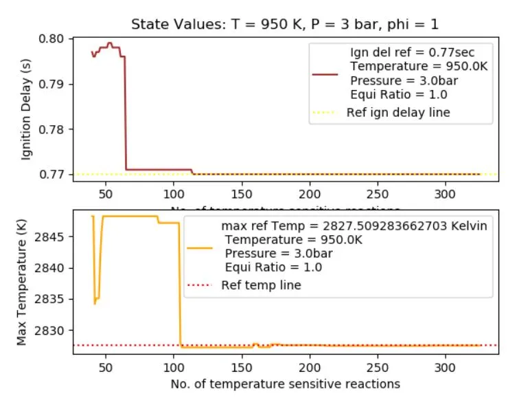
Case 2

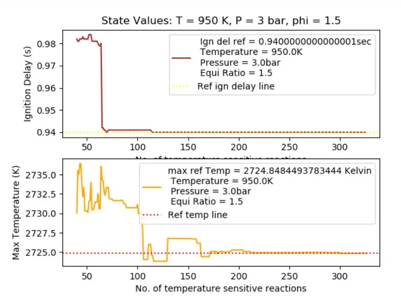
Case 3

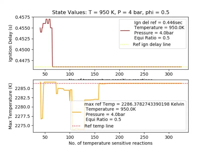
Case 4

Case 5

Case 6

Case 7

Case 8

Case 9

Case 10

Case 11

Case 12

Case 13

Case 14

Case 15

Case 16

Case 17

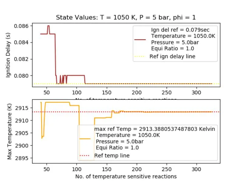
Case 18

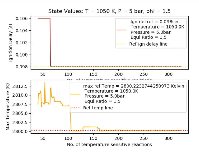
Case 19

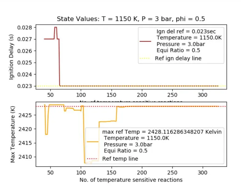
Case 20

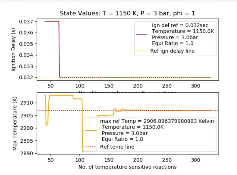
Case 21

Case 22

Case 23

Case 24

Case 25

Case 26

Case 27

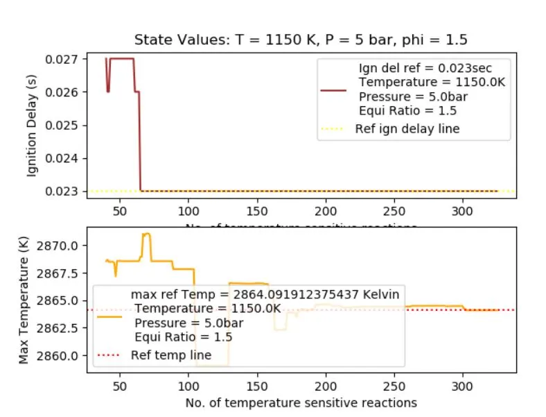
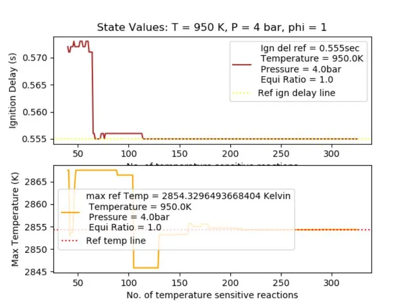
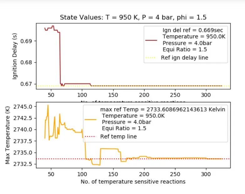
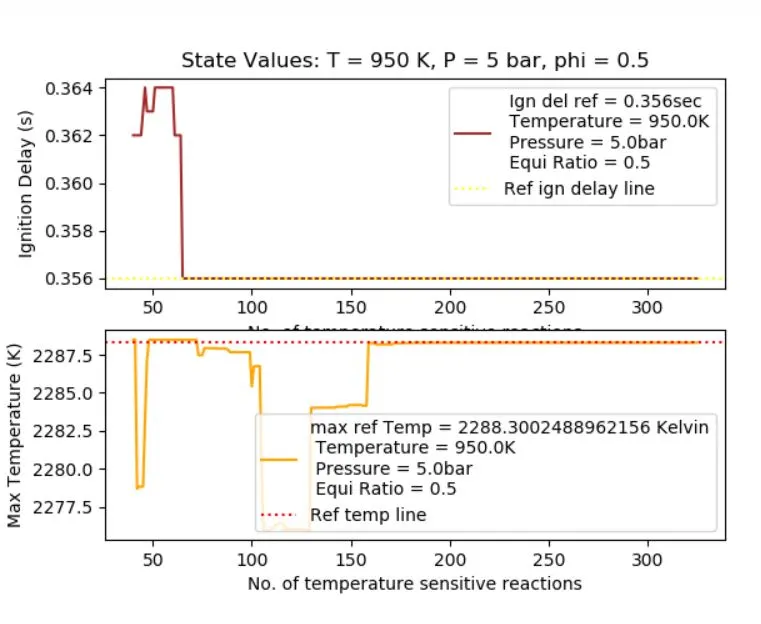
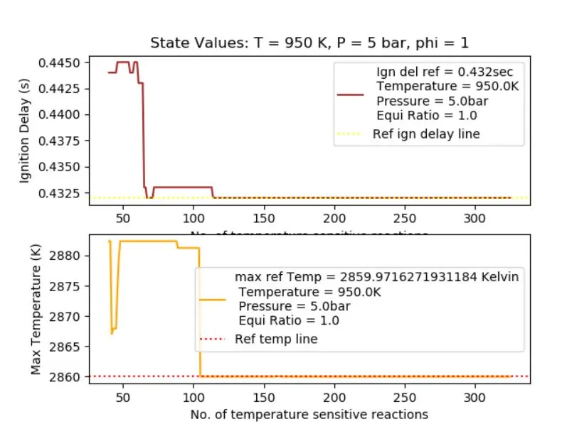
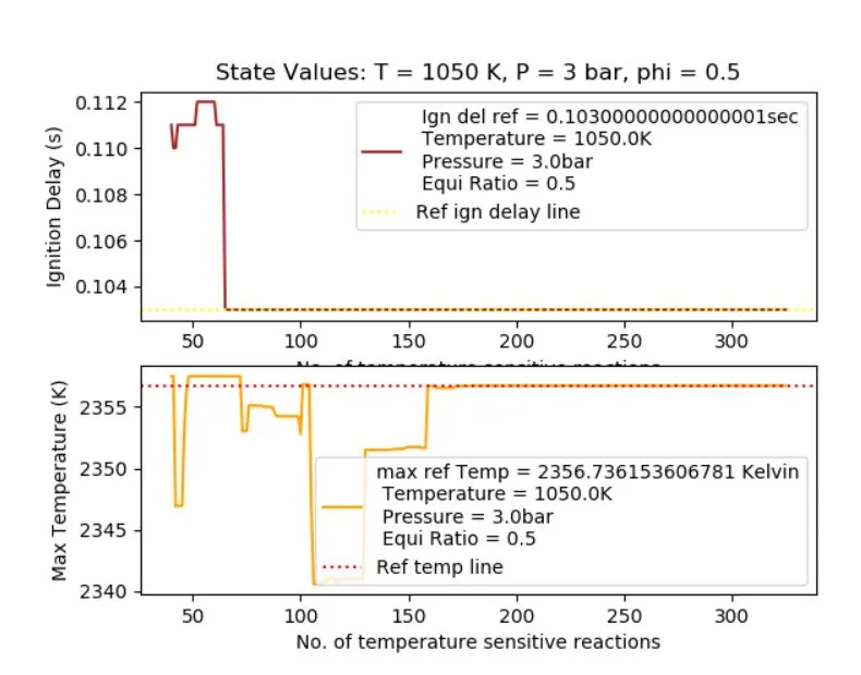
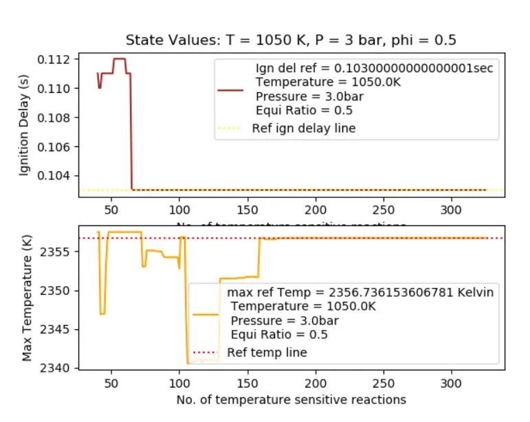
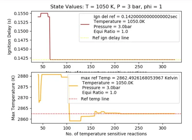
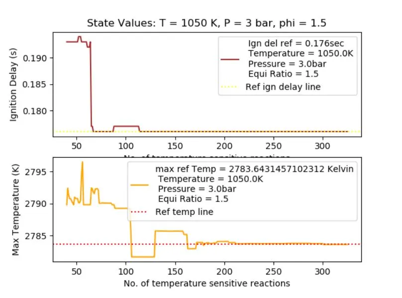
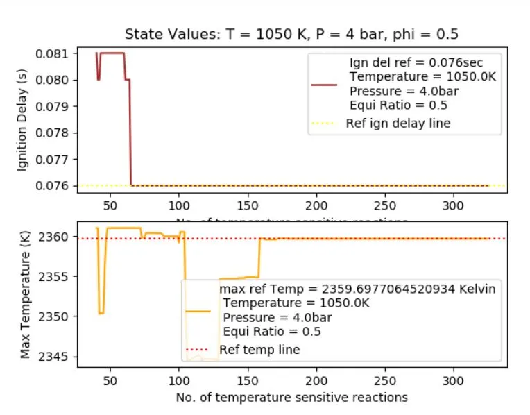
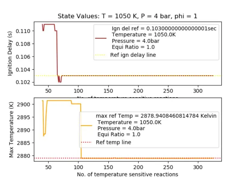
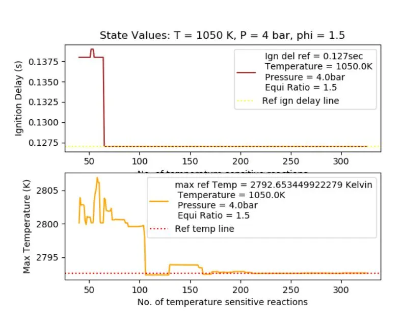
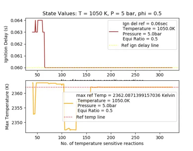
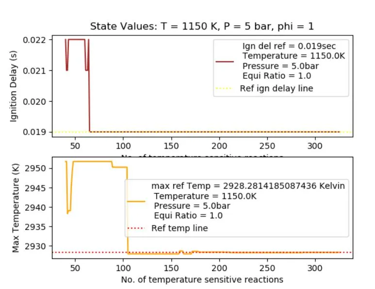
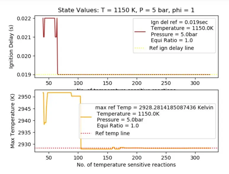
1. All the above graphs for different combinations of state values show a similar trend.
2. Both ignition delay and maximum temperature graphs show fluctuations of high magnitude initially.
3. As more and more reactions are added, the oscillations dampen and the graphs approach towards the reference values.
   We are ordering the reactions in the decreasing order of sensitivities.
4. Higher the sensitivity, lower the ignition delay and higher the maximum temperature and vice versa.
5. Therefore reactions being appended at the early stages have the highest sensitivity and hence greater influence on the ignition delay and maximum temperature.
6. That is the reason why the magnitude of fluctuations is high initially.
7. And as we append more of the less sensitive reactions, the average or the net sensitivity of the reactions gradually decreases resulting in lesser magnitudes of fluctuations and after a certain point, the graph attains a steady state.

CONCLUSION

1. Reaction mechanism was reduced based on senstivity analysis
2. Plots for the same shows the reduction of reactions from 40 to 27 critical reactions
3. There is almost no significant difference in the ignition delay of the maximum temperature behaviour