Rayleigh Taylor Instability Challenge
AIM:-
- To explain the mathematical models that have adopted for CFD calculations that are based on Rayleigh Taylior waves.
- To perform the Rayleigh Taylor instability simulation for 2 different mesh sizes with the basemesh being 0.5 mm and the other with refined mesh by water and user material(`rho`:- 400kg/m^3, `mu`:-0.001kg/m-s).
- To explain why a steady state approach might not be suitable for these type of simulations.
- Define and find out the Atwood number for the both the cases and discuss the behavior of the instability.
EXPLANATION AND SIMULATION:-
Rayleigh-Taylor Instability:-
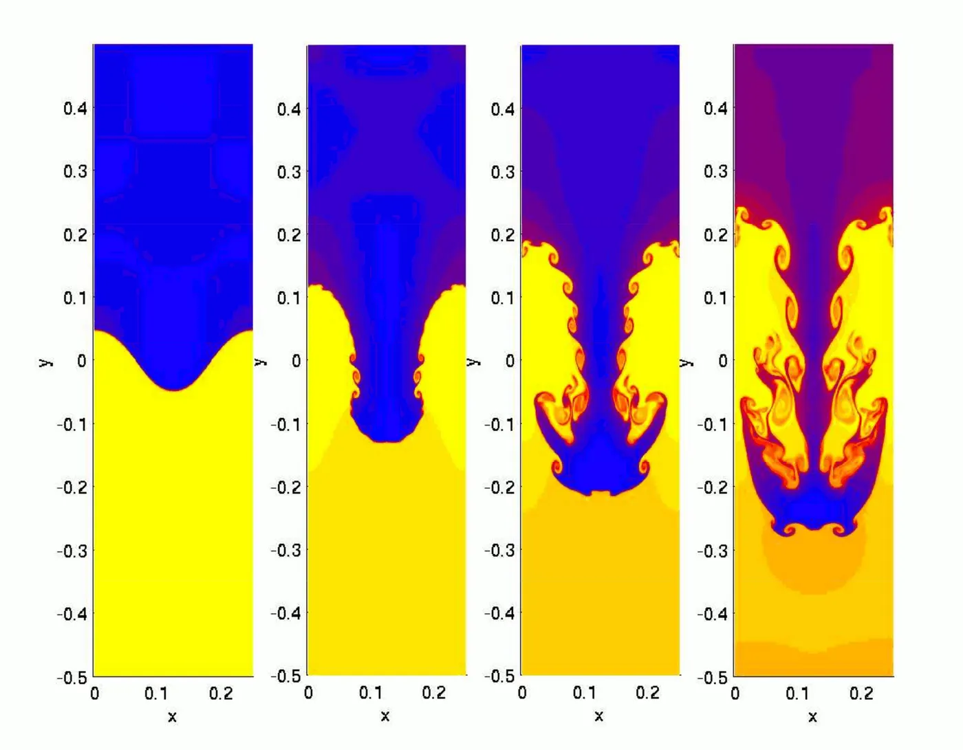
This is the instability coused when two fluids wth different densities share acommon horizontal interface.
The lighter fluid will be pushing heavier fluid to over come the instability by gravity.
In the below simulatuion we will see two different cases with digferent densities.
Some Practical CFD that are based on Rayleigh-Taylor waves:-
Richtmyer-Meshkov Instability (RMI):-
This instability occurs when two fluids of diiferent densities impulsively accelerated. Normally this is by the passage of a shock wave. The development of the instability begins with small amplitude perturbations which initially grow linearly with time. This can be seen at wide range of Mach number.
Plateau-Rayleigh Instability:-
The Plateau-Rayleigh instability, often just called the Rayleigh instability, explains why and how a falling stream of fluid breaks up into smaller packets with the same volume but less surface area. This can be seen when the rain water stream is breaking into droplets.
Kelvin Helmholtz Instability:-
The kelvin Helmholtz instabilityoccurs when there is velocity shear in a single continuous fluid, or additionally where there is a velocity difference across the interface between two fluids. We can see with wind blowing over water, the instability constant is able to manifest itself through waves on a water surface.
Now let's do the simulation:-
Geometry:-
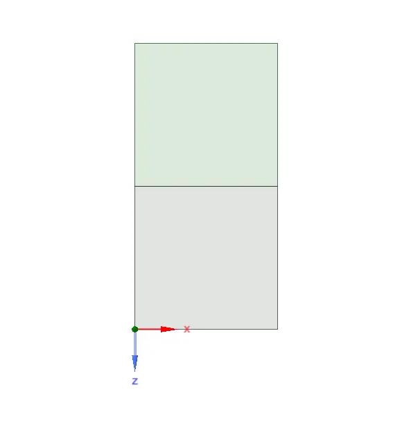
I have created two phases on the xz-plane and named them air and water respectively.
Make sure that you have 'share' the topology otherwise the information inside the phases will not pass between them.
Mesh:-
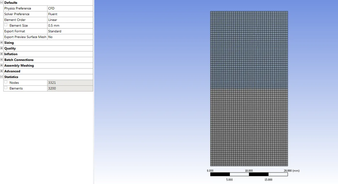
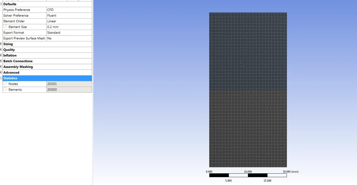
I have created three different meshes to observe how the two fluids are actually mixing and moving in the phases. As this is like a rectangular plate- elements are perfectly squared and distributed equally.
Case 1:-
This is the baseline mesh with the element size 0.5mm
Case 2:-
In this case I have refined the mesh a bit more with the element size of 0.2mm.
Case3:-
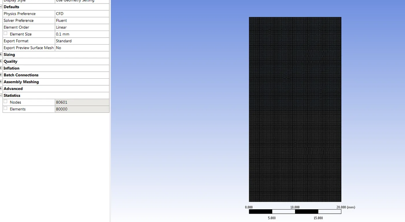
In this xasse I have refined further more with element sixze of 0.1mm.
Fluent Setup:-
I have used pressure-based, absolute velocity, trransient state solver.
I am using Transient state here instead of steady state because transient state is time dependant we want to know what is happening in between the phases as soon as the fluctuation of the fluids start. We are not intrested in the final result which can be simulated with steady state. As the Renold's number is low we are sticking with pressure based solver.
Turn on the gravity in the negative y-axis with default value '-9.81'.
In the physics turn off the energy and I used 'Laminar' model as there is no turbulence happening or there is no external pressure happening.
For this simulation I am using "Multiphase-volume of fluids-Implicit" then click on apply.
Here I am considering air as the primary phase and water as the secondary phase. So copy water-liqiud from the fluent data base for the secondary phase. Make sure that air is created by default as primary phase.
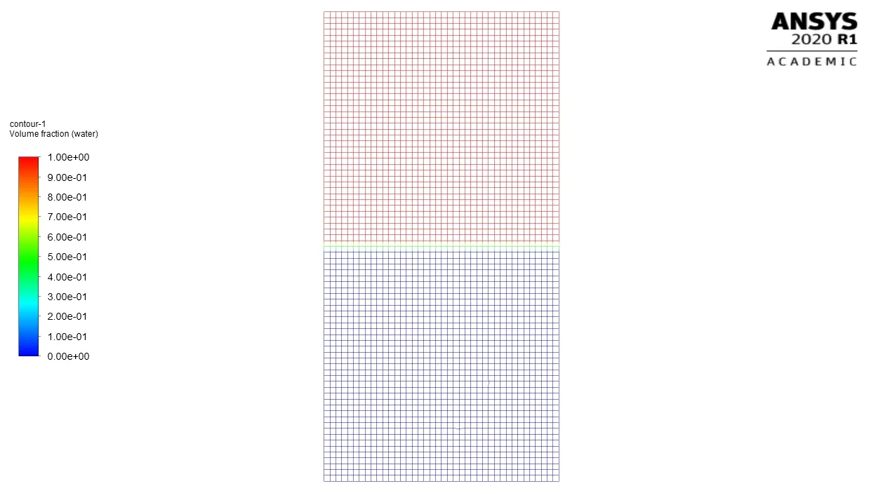
We will be using Standard initialization for this case as we have selected the transient state.
Initialize for 10 iterations and create the necessary contour and animations
Now use 'Patch' to patch the phases. Select water-volune fraction then give '1' for air and '0' for water.
Note:-Every time you initialize we have to patch that many times.
Time step:-0.005.
No.o Iteration:-
Case 1:- 150
Case 2:- 850
Case 3:- 1500
For case 1 and case 2 all the setup is same but for case 3, I have used a user-specified material (density:-400kg/m^3 and viscosity:-0.001 kg/m-s) and water.
Now let's see the Residuals and Contours.
RESULTS:-
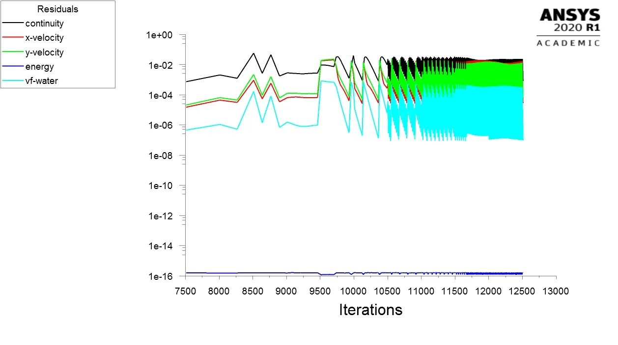
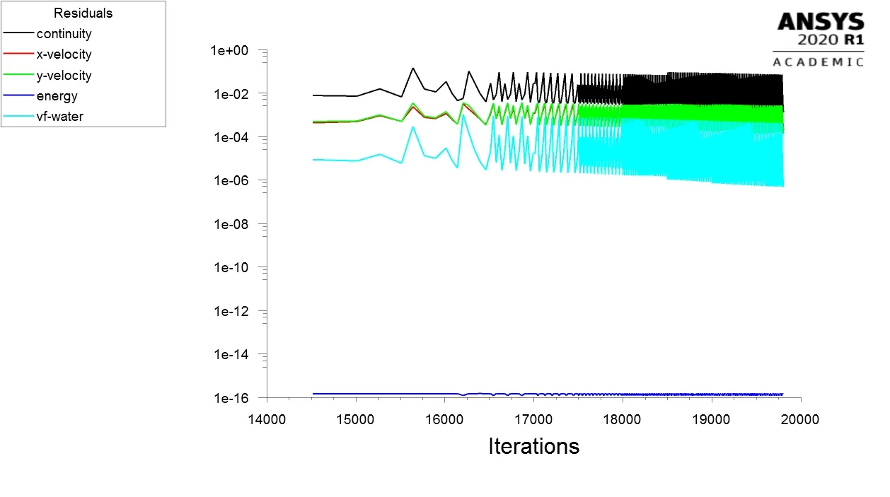
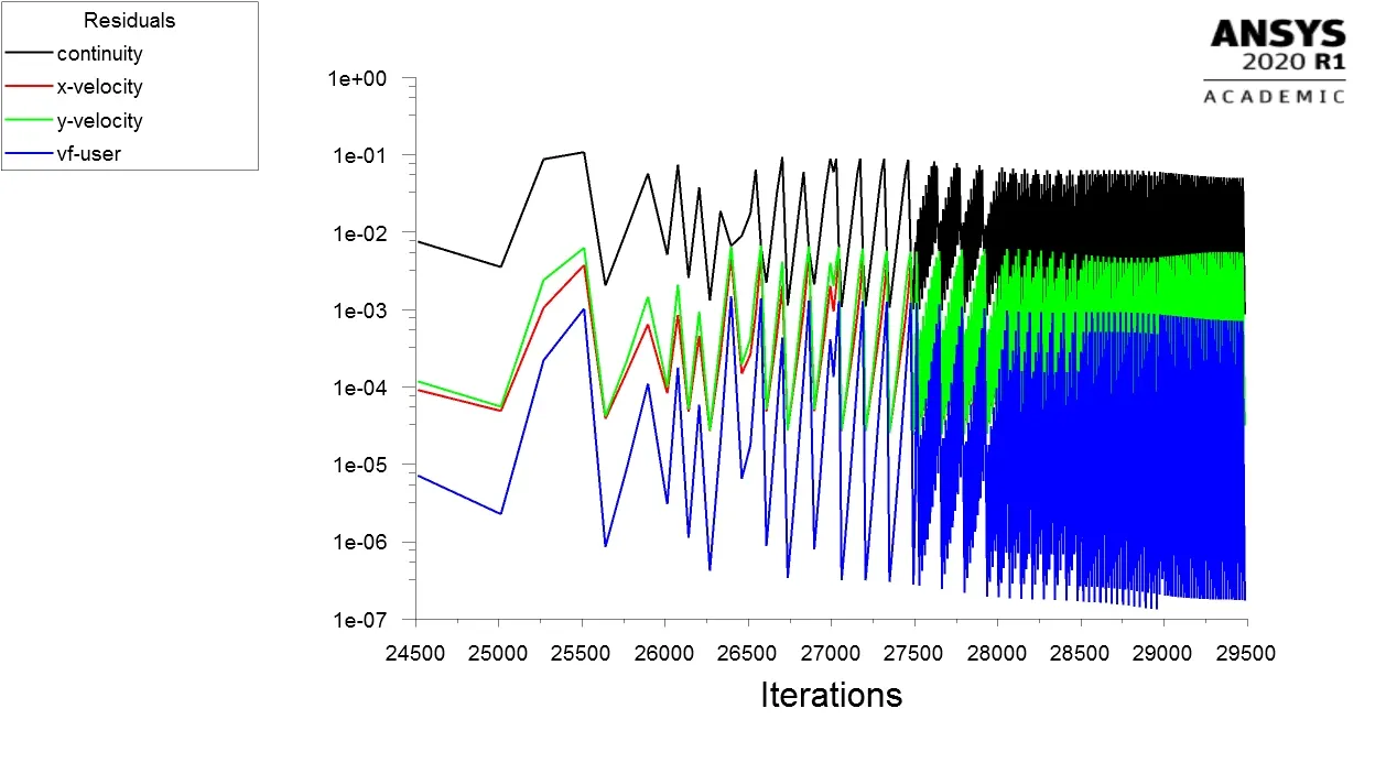
Note:- below plots are for case 1, case 2 and case 3 respectively.
Residuals:-
\
Outputs:-
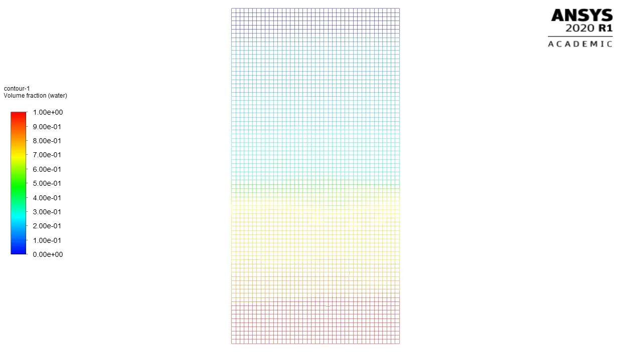
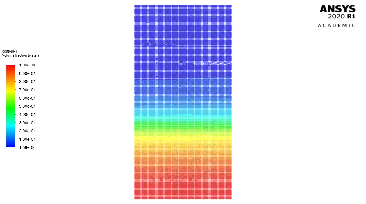
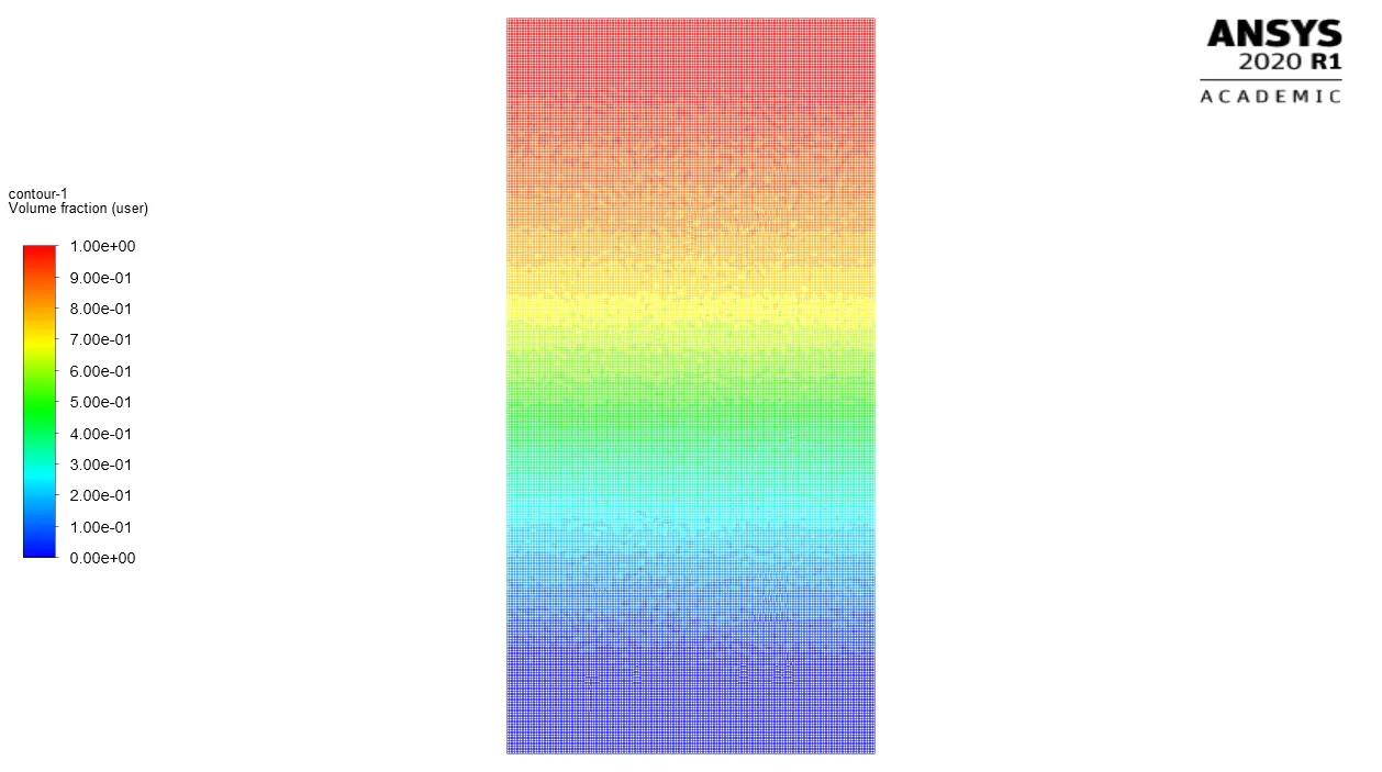
Here we can clearly see the how refined mesh is showing the physics clearly in the contours.
Now let's see the animatiobns
Case1:-
Case2:-
Case3:-
OBSERVATION:-
We can see the proper difference in the contours and animations that how the fluids are moving in between the phases. We can clearly see how bubbles and fumes in the fluids. Comapred to the case1, case 2 is pretty fine. Compared to case 2 , case 3 is more fine and better of all. But all that clear is shown with the cost of execution time.
As case 3 have a lot of cells compared to other cases more execution time is required for this simulation.
In the case 3 we can also see that the intial instability was started abit slow compared to the other cases as the case 3 fluid have more density that the other cases.
Atwood Number:-
The Atwood Number is a dimensionless number in fluid dynamics, used in the study of hydrodynamic instabilities in density stratified flows. It is a dimensionless density ratio defined as
`A= ((underset(a)rho)-(underset(b)rho))/((underset(a)rho)+(underset(b)rho))`
- A = ρ 1 − ρ 2 ρ 1 + ρ 2 {\displaystyle \mathrm {A} ={\frac {\rho _{1}-\rho _{2}}{\rho _{1}+\rho _{2}}}}
where,
`underset(a)rho`= Heavier fluid's density
`underset(b)rho`= Lighter fluid's density
- ρ 1 {\displaystyle \rho _{1}}
Atwood number is an important parameter in the study of Rayleigh–Taylor instability and Richmyer-Meshko.
In Rayleigh-Taylor instability the penetration distance of heavy fluid bubbles into the light fluid is a function of acceleration time scale
`Ag(t^2)`
A g t 2 {\displaystyle \mathrm {A} gt^{2}
where,
g is gravitational acceleration and
t is the time.
Now For the
Case1:-
where Air and Water are the fluids
Here Atwood number will be 0.9975., which is close to 1.
Case 2:-
Where Water and User-Specified fluid are the fluids.
Here Atwood number will be 0.4278, whic is close to 0.5 or 0.
Now how does the variation in Atwood number in the above two cases affects the behavior of the instability?
If the Atwood number is closer to one or more that one then the stabilization of the fluid will get decreased as there is huge density difference between the fluids. In the case 1 you can see that the Atwood number is higher compared to the case 3. So the instability was very fast in the first case.
So we can say that if the Atwood number is high fluid will get disturbed in a more stable way compared to the low Atwood number fluids. In the low Atwood number the bubbles amplitude is quite larger that the high Atwood number case.