Rayleigh Taylor Instability Challenge
Kelvin-Helmholtz Instability (KHI) is a hydrodynamic instability in which immiscible, incompressible,
and inviscid fluids are in relative and irrotational motion. In KHI, the velocity and density profiles are
uniform in each fluid layer, but they are discontinuous at the (plane) interface between the two fluids.
This discontinuity in the (tangential) velocity, i.e., the shear flow, induces vorticity at the interface; as a
result, the interface becomes an unstable vortex sheet that rolls up into a spiral. KHI is observed in a
wide rage of nature.
Applications:
Instabilities of this kind frequently occur in nature, two such manifestations are the so-called “wind-
over-water” and “clear air turbulence” instabilities.
The Plateau-Rayleigh Instability:
The Plateau-Rayleigh Instability describes the phenomenon where a falling jet or cylinder of fluid (such
as water) at one point ceases to be a jet and breaks into multiple droplets of smaller total surface area.
The short explanation for this is that the surface energy is minimized by this change. The phenomenon
is primarily one of surface tension. For this reason gravity and viscous forces are not significant and
hence are ignored.
The driving force of the Plateau–Rayleigh instability is that liquids, by virtue of their surface tension,
tend to minimize their surface area.
Applications:
1.Water dripping from a tap.
2.Inkjet Printing.
Bubble merger and scaling law:
A theoretical model to study the effects of surface tension on the growth of single and multiple bubbles
in the Rayleigh-Taylor instability. The asymptotic solution for a single bubble is obtained and is
expressed in terms of the Eotvos number.(A non-dimensional parameter that arises in the study of
bubbles and drops rising or falling in another fluid, including within a tube).
The bubble merger process is also demonstrated with the model.Results obtained were effects of
surface tension: it reduces the growth of a single bubble, but enhances the mixing rate of multiple
bubbles at a late time. The bubble merger of Rayleigh-Taylor instability follows the same scaling law of
the growth of mixing zone even when surface tension exists, but the growth coeffcient in the scaling law
increases with surface tension.
Rayleigh Taylor instability:
The Rayleigh-Taylor instability takes place when a heavy fluid is situated above a light fluid in a
gravitational field pointing toward the light fluid. The interface becomes unstable for certain perturbation
wavelengths and these perturbations evolve into bubbles of light fluid and spikes of heavy fluid which
penetrate into both fluids. The evolution of a Rayleigh-Taylor (RT) unstable interface is complex,involving
phenomena such as the development of a Helmholtz instability on the side of the penetrating spikes,
formation and detachment of droplets, competition and amalgamation among rising bubbles,
entrainment and turbulent mixing in a region of fluid of finite thickness, and a possible chaotic limit with
a fractalized interface. Therefore, the Rayleigh-Taylor instability is the prototype case for fluid mixing
induced by unstable stratification, and as such, is of fundamental importance; it has been the subject of
numerous experimental and numerical studies in fundamental research and practical applications such
as multiphase hydrodynamics.
The Rayleigh-Taylor instability occurs in diverse applications, including: the electromagnetic implosion of
a metal liner, the formation of high luminosity twin-exhaust jets in rotating gas clouds in an external
gravitational potential, the overturn of the outer portion of the core of a massive star, and the laser
implosion of deuterium-tritium fusion targets in inertial fusion systems. Rigorous understanding of these
phenomena can be gained by investigating the Rayleigh-Taylor instability.
##Solving And Modelling Approach:
Geometry preparation in Spaceclaim.
Meshing in Mesh tool
In Setup-Setting up case including solver,Turbulence Model,boundary condition etc.
Post process results.
We will discuss three cases-
First two using Air and water as materials:
1.Base Mesh (0.5 mm element size)
2.Refined Mesh(-- element size)
Third case using water and a user defined material:
3.Refined Mesh(-- element size)
#Pre processing,Solver settings:
Case-1:
#Geometry:
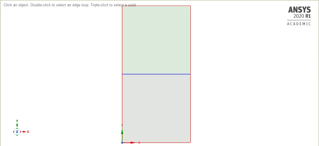
Create 2D two components in Spaceclaim,
one for air and other for water volume.
For say Air,create rectangle of 20mm x 20mm dimensions.
Use Pull tool,
Then do same for water and create water volume above Air volume.
Share both component Topology by share tool.
#Meshing:
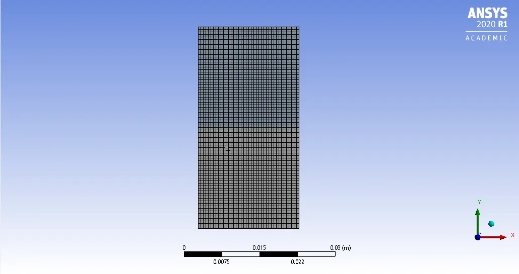
Element size-0.0005 m.
Total no of cells-3200
#Setup:
Solver used Transient with inclusion of Gravity effect.
Viscous model used-Laminar.
In Multiphase Model:
Select Volume of fluid model,
Volume fraction formulation-Implicit.
Set materials in Multiphase model;
Water for Upper volume,
Air for lower volume.
Standard Initialization of Solution ,
Then Create Patch for Volume fraction.(Value we are setting is actually value of `alpha`.In volume of fluid method if `alpha`=1 indicate different phase and `alpha`=0 indicate different phase.
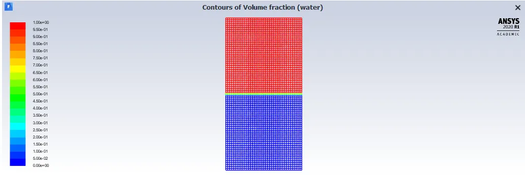
Upper volume set water and value equal to 1.
Lower volume set air and value equal to 0.
Create contour for Phase and its Animation file too.
Run calculation for 500 iterations and time step size of 0.005.
#Results:
1.Contour of Volume fraction after Initialization of solution:
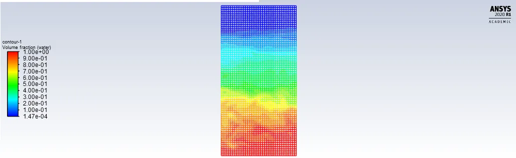
2.Contour of Volume fraction obtained after completion of 500 iteration with time step size of 0.005:
#Link to the animation of Simulation:
https://drive.google.com/file/d/18EhrJkcFaaZyD0t-sSYrmF8KRm3lVePM/view?usp=sharing
Case-2:
#Geometry:
Prepared in same way as in previous case.
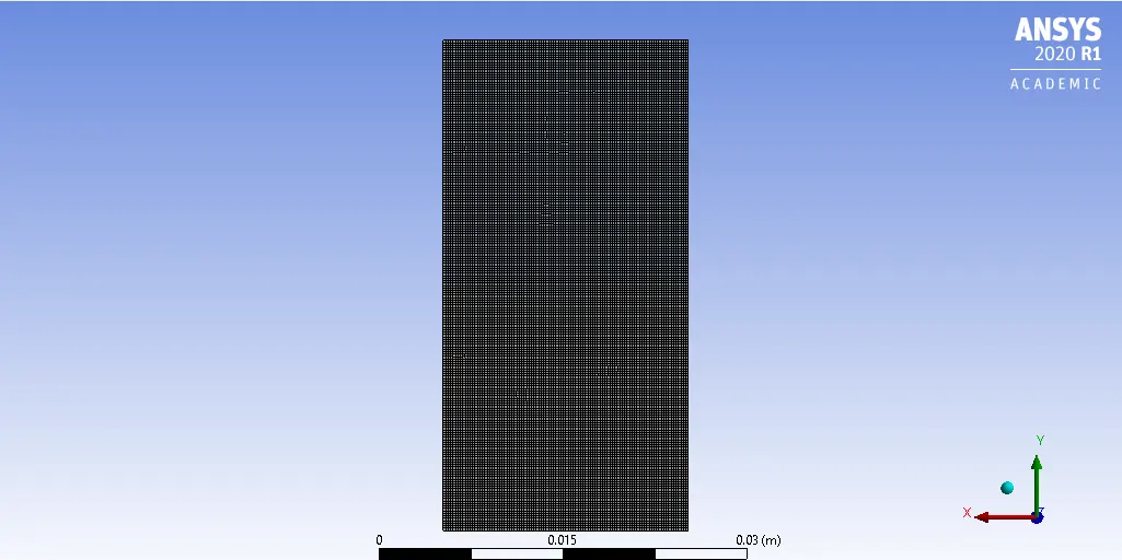
#Meshing:
Element size-0.0002 m
Total No of cells:20000
#Setup:
Solver used Transient with inclusion of Gravity effect.
Viscous model used-Laminar.
In Multiphase Model:
Select Volume of fluid model,
Volume fraction formulation-Implicit.
Set materials in Multiphase model;
Water for Upper volume,
Air for lower volume.
Standard Initialization of Solution ,
Then Create Patch for Volume fraction.(Value we are setting is actually value of `alpha`.In volume of fluid method if `alpha`=1 indicate different phase and `alpha`=0 indicate different phase.
Upper volume set water and value equal to 1.
Lower volume set air and value equal to 0.
Create contour for Phase and its Animation file too.
Run calculation for 500 iterations and time step size of 0.005.
#Results:
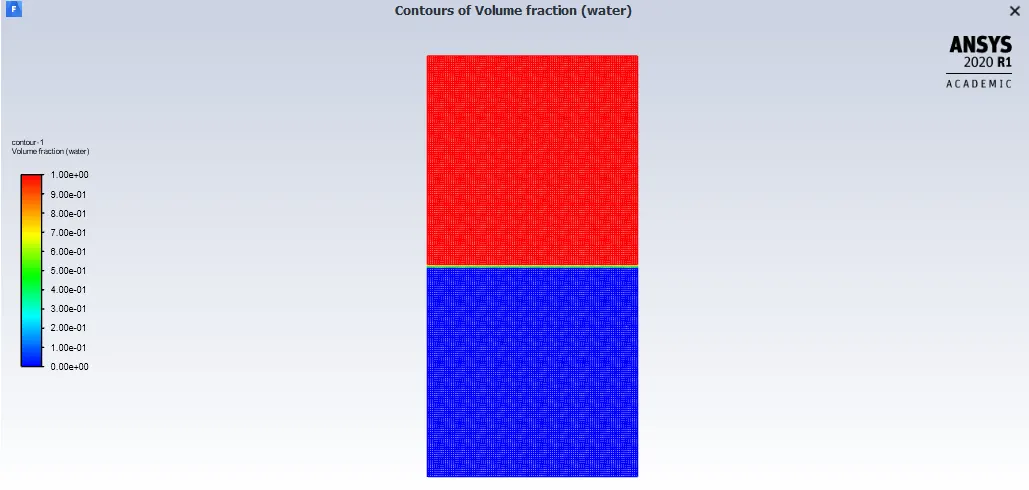
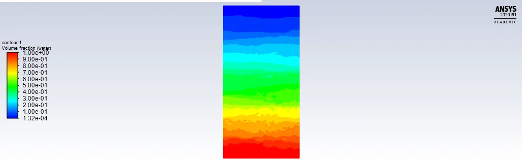
#Link to the animation of Simulation:
https://drive.google.com/file/d/1nCtBvxr7OnnhyRmIh7Km5uf16sqFQ8CW/view?usp=sharing
Case-3:---(density=400`(kg)/m^3`;viscocity=0.001 `(kg)/(m-s)`)
#Geometry:
Prepared in same way as in previous case.
#Meshing:
Element size-0.0002 m
Total No of cells:20000
#Setup:
Solver used Transient with inclusion of Gravity effect.
Viscous model used-Laminar.
In Multiphase Model:
Select Volume of fluid model,
Volume fraction formulation-Implicit.
Set materials in Multiphase model;
Water for Upper volume,
User defined material for lower volume.(density=400`(kg)/m^3`;viscocity=0.001 `(kg)/(m-s)`)
Standard Initialization of Solution ,
Then Create Patch for Volume fraction.(Value we are setting is actually value of `alpha`.In volume of fluid method if `alpha`=1 indicate different phase and `alpha`=0 indicate different phase.
Upper volume set water and value equal to 1.
Lower volume set user defined and value equal to 0.
Create contour for Phase and its Animation file too.
Run calculation for 900 iterations and time step size of 0.001.
#Results:
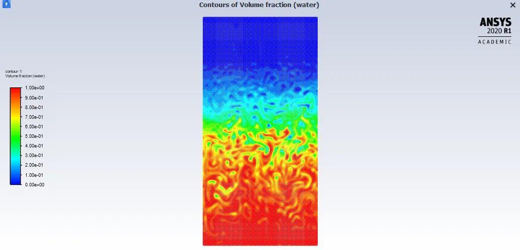
#Link to the animation of Simulation:
https://drive.google.com/file/d/1BJVZQ5tGl0GQmlE3QCInMOZC_EHV48lt/view?usp=sharing
#Effect of Mesh size on simulation:
By setting same case setup for both cases 1 and 2 except mesh sizes are different
For case-1 -Mesh size-0.0005 m
For case-2 -Mesh size-0.0002 m
Both cases simulation giving i think same results,only difference lies in capturing results more
accurately.
In coarse mesh(Case 1)-Not much spike ,or sinusoidal shape not generated at interface.It only lead to
bubbles formation,then growth of Mushroom structure and at last turbulent mixing happened very late.
In Refined mesh(Case-2)-More spike and sinusoidal shape generated at interface.Bubbles formation
captured more clearly,then how it detached and lead to Mushroom structure formation.Turbulent mixing
at the end is captured very accurately.
#Why a steady-state approach might not be suitable for these types of simulation:
Steady state approach is used where we are studying a phenomenon which is not changing with
time.Like studying a aerodynamic effect around car body can be done with Steady state approach
though better results will be obtained with Transient approach.But still it can be used.
Transient approach is used for studying phenomenon where changes are taking place with respect to
time.Like this case Rayleigh Taylor Instability phenomenon,here two fluid are at rest and separated by
interface.The interface becomes unstable for certain perturbation wavelengths and these perturbations
evolve into bubbles of light fluid and spikes of heavy fluid which penetrate into both fluids. This
instability is changing and taking place with respect to time,after sometime it will become stable.Lighter
fluid will reach on top and heavier fluid in the bottom.
Atwood Number:
The Atwood number (A) is a dimentionless number in fluid dynamics used in the study of hydrodynamics instabilities in density stratified flows. It is a dimensionless density ratio defined as
- `A=(rho_1-rho_2)/(rho_1+rho_2)`
where
- `rho_1`= density of heavier fluid
- `rho_2`= density of lighter fluid
Atwood number calculation for Case-2 and Case-3:
Case-2
As `A=(rho_1-rho_2)/(rho_1+rho_2)`
`rho_1`= density of heavier fluid=997`(kg)/m^3`
`rho_2`= density of lighter fluid=1.225`(kg)/m^3`
`A=(997-1.225)/(997+1.225)`
A=0.9975
Case-3
As `A=(rho_1-rho_2)/(rho_1+rho_2)`
`rho_1`= density of heavier fluid=997`(kg)/m^3`
`rho_2`= density of lighter fluid=400`(kg)/m^3`
`A=(997-400)/(997+400)`
A=0.4273
#Effect of variation in Atwood number in the above two cases affects the behavior of the
instability. :
From Case 2 and Case 3 where Atwood number is 0.9975 and 0.4273 respectively.What we observed:
Case-2
As difference between density of heavier and lighter fluid is very high and also Atwood number is high. In the early stage, a sinusoidal initial perturbation retains its sinusoidal shape
After this stage ,one observes the beginnings of the formation of the ubiquitous mushroom-shaped spikes (fluid structures of heavy fluid growing into light fluid) and bubbles (fluid structures of light fluid growing into heavy fluid).The growth of the mushroom structures continues in the second stage.
The spikes and bubbles then begin to interact with one another in the third stage. Bubble merging takes place, where the nonlinear interaction of mode coupling acts to combine smaller spikes and bubbles to produce larger ones. Also, bubble competition takes places, where spikes and bubbles of smaller wavelength that have become saturated are enveloped by larger ones that have not yet saturated. This eventually develops into a region of turbulent mixing,which is the fourth and final stage in the evolution.
Case-3
Difference between density of heavier and lighter fluid is very less and also Atwood number is low.
In this case due to less difference in densities ,we missed sinusoidal shape and amplitude of spikes generated are less and spikes are less in number.Bubble formation and interaction of spike and bubble takes place very fast.Growth of Mushroom structure takes place and at the end Turbulent mixing.