Rayleigh Taylor Instability Challenge

OBJECTIVES

1. To understand Rayleigh Taylor instability and some CFD models that have been based on the mathematica analysis of Rayleigh Taylor waves.
2. To perform the Rayleigh Taylor Instability simulation for different mesh sizes and compare them.
3. To find out the affect of Atwood number variation on Ryaleigh Taylor Instability.

INTRODUCTION

Rayleigh Taylor instability is the phenomenon where the two fluids of different densities interact with each other. When the light fluid pushes the heavy fluid toward each other or the two fluids seek to reduce their combined potential energy.

RTI has many practical effects on the Earth's climate and many other real life examples such as mixing of oil and water, mushroom clouds after the volcanic eruption. Apart from that the winds off the coast of greenland and iceland drive the evapouration from the upper surface of teh oceans making the upper layers heavier. This in turn generates the absyyal ocean circulation which acts as the heat pump tansporting the warm waters to up north thus protecting the nothern europe from drastic drop in temperature.

RTI at the interface of the plane of two fluids and when the heavier fluid is above the lighter fluid and under the influence of gravitational force the shock wave is generated in teh fluid and the hravier fluid starts the come down and at the same time the lighter fluid starts to move up in the form of bubbles. These bubbles are formed due to the surface tension of the heavier force which applies the force on teh inrerfacing plane of teh lighter fluid thus forming them in bubbles and moving up.

Some practical applications of the RTI are in the jet engine where the fuel comes in the form of spray which in turn converted into tiny droplets due to RTI and thus increase the surface area to increase the combustion process.

Some CFD applications of RTI.

1.)Richtmyer–Meshkov instability

The Richtmyer-Meshkov instability occours when the two fluids of different densities are impulsively acclerated towards each other. This is generally done by the shock wave. The instability starts with small amplitude pertubations which grow with the time.This is followed by a nonlinear regime with bubbles appearing in the case of a light fluid penetrating a heavy fluid, and with spikes appearing in the case of a heavy fluid penetrating a light fluid. A chaotic regime eventually is reached and the two fluids mix.

2.)Plateau–Rayleigh instability

The Plateau–Rayleigh instability, often just called the Rayleigh instability, explains why and how a falling stream of fluid breaks up into smaller packets with the same volume but less surface area. It is related to the rayleigh taylor instability and is part of a greater branch of fluid dynamics concerned with fluid thread breakup. This fluid instability is exploited in the design of a particular type of ink jet techonology whereby a jet of liquid is perturbed into a steady stream of droplets.

3.)Kelvin–Helmholtz instability

The Kelvin–Helmholtz instability typically occurs when there is velocity shear in a single continous fluid, or additionally where there is a velocity difference across the interface between two fluids. A common example is seen with wind blowing over water, the instability constant is able to manifest itself through waves on a water surface. The Kelvin-Helmholtz instability is not only restricted to a water surface as clouds, but is evident through other natural phenomena as the ocean, Saturn's bands, jupiter's red spot, and the sun's corona.

Methodology

1. Modeling
2. Meshing
3. Pre-Processing
4. Solving
5. Post-Processing

1. Modeling

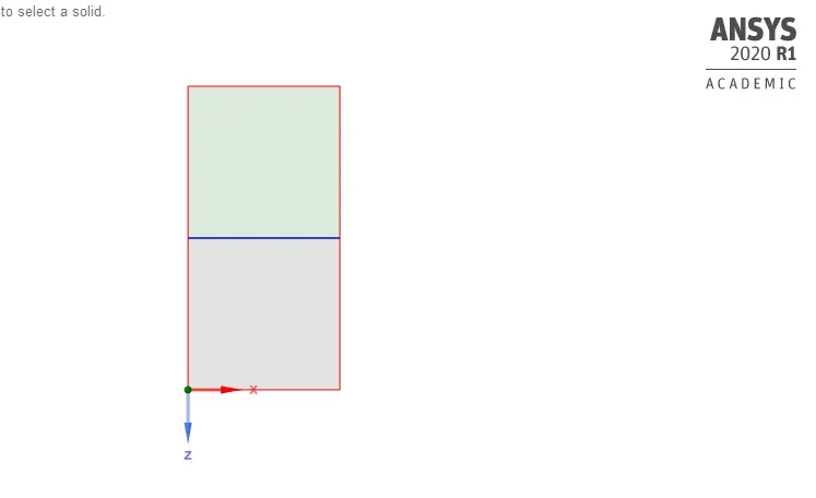
First of all we will create the a rectangular volume of 20x20 in ANSYS spaceclaim and we will name it as the air and further we will again create the rectangular volume again 20x20 mm above the air volume and further name it as water and further we will enable the shared topology.

2. Meshing

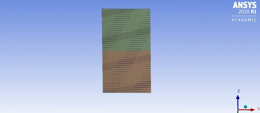
First, we will create the baseline 2d mesh and we will set the solver and then we will check the results again for the redefined mesh to get much better and appropriate results. But further when we redefine the mesh we need to check the mesh quality and further reduce the time step size to keep the CFL number below 1.

Mesh	Element Size	No of Elements
Baseline Mesh	0.5mm	3200
Refinment 1	0.25	12358
Refinement 2	0.125	55438

3. Setting up the Physics (Pre-processing)

For this type f simulation the transient simulation has been chosen because we want to study the mixing of the fluid and how the phenomenon takes place rather than the end result or the steady state result.

Solver: Pressure Based Solver

Velocity: Absolute Veocity

Gravity has been enables to check the mixing as the water is above the air in initiaal conditionsthus the gravity is give in -ve y direction .i.e. -9.81.

As the fluids have no relative high velocities or the the reynolds umber is low thus we will be working with laminar flow model.

Clearly here we are working with the two different phases of fluid thus we will be working with the multiphase mode with 2 eularian fluids. We will be solving this problem implicitly because in explicit model the CFL criteria has to be taken into consideration thus finding the accurate value of delta t will be quite difficult .

Materials we will be working with the two materials that is air and water. Further we will be working with the coupled implicit solver and further will be working with the first order upward scheme.

Further we will be initializing the solution with the standard solution and we will patch volume according to the volume fraction in the relative errors. Here we will patch the air with the volume fraction of 0 and the water with the volume fraction of 1.

4.) Solving

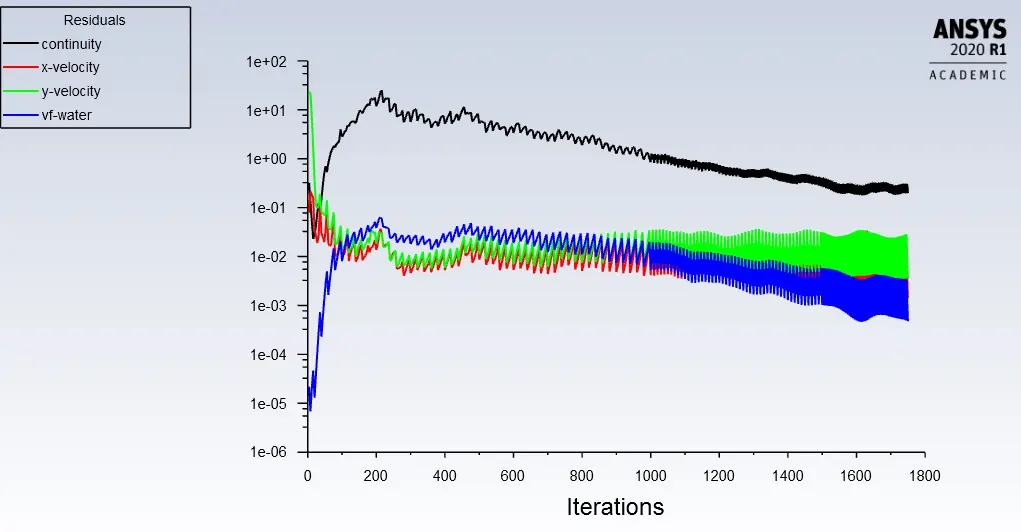
For the mesh size of 0.5mm the residual plot can be seen below:

The results can be seen below with the given link as

https://drive.google.com/file/d/1mzEacLbo1fZupy_nuRmrZ0Pz-znu-YV4/view?usp=sharing

b) Mesh size 0.25mm the results can be seen below in the given link

https://drive.google.com/file/d/17n39iw1GIL7rorNwaOPQkxNHhwbAbIE4/view?usp=sharing

c) Mesh size 0.125mm the results can be seen below in the given link

https://drive.google.com/file/d/1wAeM5QCQRR6wGERq_0_B-jNWK58C2RWw/view?usp=sharing

Case 2 : Primary Phase- Air

Secondary Phase- User Defined

Density- 400kg/m3, viscosity-0.001kg/M-S.

Further,

a). Mesh Size 0.5mm the results caan be seen below:

https://drive.google.com/file/d/1rZhoUjTIPBMzV3Pl2Qy_Lm4qM2NhWRYg/view?usp=sharing

b). Mesh Size 0.25mm the results caan be seen below:

https://drive.google.com/file/d/1GsKgJPIA5eUeIsAOTS16vWf-VgSFLYRX/view?usp=sharing

c). Mesh Size 0.125mm the results caan be seen below:

https://drive.google.com/file/d/1kNEQMDw0dAN7aHixeBTbli6btb1nV8RC/view?usp=sharing

Result:

As we reduced the mesh size for the successive simulations we get the good distribution of the instability in the cases. The mixing is more perfect and good and the boundary layers mix better when we increase the mesh size. Further if we decrease the mesh size and go for the finer mesh the computational time incrreases and teh time step size has also to be taken into consideration. Further if we decrease teh time step to too low size the computational size will increase a lot.

As explained above the steady state approach is not suitable for this simulation because we are interested in studying the process of mixing in the Reyligh Taylor Instability. As the mixing process is function of time the transient analysis will give the better results and will give the process at specific time in the process. Further we are not intersted in the last steady state result we will go with the transient state simulation.

Atwood Number

Atwood numbr is a dimentionless number in the fluid dynamics is used to study teh hydrodynamics instabilities. It is a very important parameter to study the Reyleigh- Taylor instability. Atwood number can be give by the formula shown below:

A={Density of heavier fluid-Density of lighter fluid}/{Density of heavier fluid+Density of lighter fluid}

or it can be given by

`A=frac{rhounderset(1)( )-rhounderset(2)( )}{rhounderset(1)( )+rhounderset(2)( )}`

Case 1: Atwood Number=0.99775, as we can see that the A is near 1 the vortses produced will be less and teh steady state will reach in a lesser time.

Case 2: Atwood Number = 0.422, we get the more vortecies in the simulation thus resulting in more turbulence.

Inference:

Transient simulation is used here because we want to study the process of the mixing of fluids and how will they behave before going to the steady state thus a transient simulation is used to study the rayleigh instability.

The process is directly affected by the mesh size thus when we use the finer mesh we can see the good distribution in the instability and we can capture the better turbulence but decresing the mesh size will also reduce the time step size and thus also increse the computational time.

Here in the formula we can see that the atwood number depends upon the densities and should be in the range of 0-1.

Here we can see that the atwood number for air water mixing is near to 1 thus the mixing is quiet fast and takes less time to come to steady state. For water aand the user defined material the mixing is alow and takes the larger time to come to the steady state.