Rankine Cycle

AIM: To create a Rankine cycle simulator and to find out the thermodynamic properties at each state.

OBJECTIVES OF THE PROJECT:

1. To calculate the state points of the Rankine Cycle.

2. To plot the T-S and H-S plots for the given inputs.

3. To calculate the Net work output and Back work ratio.

RANKINE CYCLE

• The Rankine cycle is a thermodynamic representation of a high-pressure or expansion type of steam engine cycle, and because of the shape of the T-s saturation curve for water, the ideal or reversible Rankine cycle.
• without superheat is very close to the (reversible) Carnot cycle.
• It is very difficult to efficiently pump wet vapour back into the boiler in the
  Rankine cycle, the vapour is completely condensed into a liquid in the condenser and, using a common liquid pump, pumped into the boiler as a compressed liquid.
• The Rankine cycle boiler feed pump raises the pressure of the liquid condensate to only that of the boiler, leaving its temperature nearly equal to that of the
  condenser.
• Processes

1 → 2: isentropic expansion in a turbine,
2 → 3: isobaric cooling in a condenser,
3 → 4: isentropic compression in a pump, and
4 → 1: isobaric heating in a boiler.

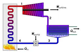
STEADY FLOW ENERGY EQUATION:

`(u_1+p_1*v_1+Z_1*g+C_1^2/2)+Q=(u_2+p_2*v_2+Z_2*g+C_2^2/2)+W`

where, Q=Heat supplied per kg of fluid,

W=Work done by 1kgof fluid,

C = Velocity of fluid,

Z= Height above datum,

p=Pressure of the fluid,

u=Internal energy of per kg of fluid, and

pv=Energy required for 1kg of fluid.

Applying study flow energy equation(S.F.E.E) to boiler, turbine, condenser and pump :

• for boiler: `Q_1=h_1-h_(f4)`
• for the turbine: `W_T=h_1-h_2`
• for condenser: `Q_2=h_2-h_(f3)`
• for the feed pump: `W_P=h_(f4)-h_(f3)`
• Efficiency of ranking cycle: `η=(W_T-W_P)/Q_1` `

`η=((h_1-h_2)-(h_(f4)-h_(f3)))/(h_1-h_(f4))`

• Power plants are sometimes characterized by their
• back work ratio: bwr, the ratio of pump work to turbine work.
  Here,
  bwr =pump work/turbine work

`bwr== W_P/W_T`

The programming language used: MATLAB

%%  RANKINE CYCLE 
disp('                                 RANKINE CYCLE SIMULATOR          ')
disp('  ')
fprintf(['process 1-2: isentropic expansion in the turbine \n' ...
           'process 2-3: constant pressure, transfer of heat in the condenser \n' ...
           'process 3-4: isentropic pumping process in the feed pump \n'...
           'process 4-1: constant pressure tranfer of heat inn the boiler \n'])
%%  finding the states
disp('  ')
%giving the inputs
T_1=input('Enter the Turbine inlet temperature(in  °C):  \n');
p_1=input('Enter the Turbinne inlet pressure(in bars): \n');
p_2=input('Enter the Condenser inlet pressure (in bars):  \n');

%we need 2independent, intensitive properties to define any state
%state 1(p,T)
p_1;
T_1;
%s_pT	Specific entropy as a function of pressure and temperature 
s_1=XSteam('s_pT',p_1,T_1);
%h_pT	Entalpy as a function of pressure and temperature.
h_1=XSteam('h_pT',p_1,T_1);


%state 2(p,s)
p_2;
s_2=s_1;   %isentropic expansion
%T_ps	Temperture as a function of pressure and entropy
T_2=XSteam('T_ps',p_2,s_2);
%h_ps	Entalpy as a function of pressure and entropy.
h_2=XSteam('h_ps',p_2,s_2);
%vL_p 	Saturated liquid volume
v_f=XSteam('vL_p',p_2);

%state 3(p,)
%wet vapour(2 pahse mixture) is converted to saturated liquid
p_3=p_2 ; %isobaric process
%Tsat_p	Saturation temperature
T_3=XSteam('Tsat_p',p_3);
%sL_p	Saturated liquid entropy
s_3=XSteam('sL_p',p_3);
%hL_p	Saturated liquid enthalpy
h_3=XSteam('hL_p',p_3);

%state 4(p,s)
p_4=p_1; %isentropic process
s_4=s_3;
T_4=XSteam('T_ps',p_4,s_4);
h_4=XSteam('h_ps',p_4,s_4);
%%  printing the outputs
disp('-----------------------------------RESULTS-------------------------------------------')
fprintf(['At state point 1: \n'...
           '   P1 is : %2.2f bar \n' ...
           '   T1 is : %f °C \n' ...
           '   H1 is : %f kJ/kg  \n' ...
           '   S1 is : %f kJ/kgK \n'],p_1,T_1,h_1,s_1 )
fprintf(['At state point 2:  \n'...
           '   P2 is : %2.2f bar  \n' ...
           '   T2 is : %f °C \n' ...
           '   H2 is : %f kJ/kg \n' ...
           '   S2 is : %f kJ/kgK  \n'],p_2,T_2,h_2,s_2 )
 fprintf(['At state point 3: \n'...
           '   P3 is : %2.2f bar \n' ...
           '   T3 is : %f °C \n' ...
           '   H3 is : %f kJ/kg \n' ...
           '   S3 is : %f kJ/kgK \n'],p_3,T_3,h_3,s_3 )
fprintf(['At state point 4: \n'...
           '   P4 is : %2.2f bar \n' ...
           '   T4 is : %f °C \n' ...
           '   H4 is : %f kJ/kg \n' ...
           '   S4 is : %f kJ/kgK \n'],p_4,T_4,h_4,s_4 )
  %% calculating work,efficiency,bwr
  W_t=h_1-h_2;
  %W_p=v_f*(p_1-p_2)*100
  W_p=h_4-h_3;
  W_net=W_t - W_p;
  %efficency
  Q_in=h_1-h_4;
  efficiency=W_net/Q_in;
  %Back Work Ratio
%The fraction of the work produced by the turbine that is consumed by the compressor.
%bwr =|pump work|/|turbine work|
  bwr=W_p/W_t;
  disp('  ')
  fprintf(['W_t is :  %f kJ/kgK \n'...
               'W_p is  : %f kJ/kgK \n' ...
               'Back Work Ratio  is :%f \n'...
               'Net Work Output  is : %f kJ/kgK \n'...
               'Q_in is : %f kJ/kg \n'...
               'Efficiency is : %f % '],W_t,W_p,bwr,W_net,Q_in,efficiency)
               
 %% PLOTTING


%pressure is constant along this path 

s_5=XSteam('sL_p',p_1);
h_5=XSteam('hL_p',p_1);
T_5=XSteam('Tsat_p',p_1);

s_6=XSteam('sV_p',p_1);
h_6=XSteam('hV_p',p_1);
T_6=T_5;

% saturated liquids
%staurated vapours
%critical temperature of the water is 373.946
temperature=linspace(1,374,500);

for i=1:length(temperature)
    %sL_T	Saturated liquid entropy
    s_l(i)=XSteam('sL_T',temperature(i));
    %sV_T	Saturated vapour entropy
    s_v(i)=XSteam('sV_T',temperature(i));
    %hV_T	Saturated vapour enthalpy
    h_v(i)=XSteam('hV_T',temperature(i));
    %hL_T	Saturated liquid enthalpy
     h_l(i)=XSteam('hL_T',temperature(i));
end
% T-S diagram 
figure(1)
% creating the vapor dome for T-S
plot([s_l,s_v],[temperature,temperature],'b')

hold on

%variation of entropy (4-1 isobaric process)
%in liquid region
temp=linspace(T_4,T_5,500);
s_var1=0;
for i=1:length(temp)
    %s_pT	Specific entropy as a function of pressure and temperature 
    s_var1(i)=XSteam('s_pT',p_1,temp(i));
end
%in vapour region
temp2=linspace(T_6,T_1,500);
s_var2=0;
for i=1:length(temp)
    %s_pT	Specific entropy as a function of pressure and temperature 
    s_var2(i)=XSteam('s_pT',p_1,temp2(i));
end

plot([s_1,s_2,s_3,s_4],[T_1,T_2,T_3,T_4],'ro','MarkerFaceColor','r')
text(s_1,T_1,'   1');
text(s_2,T_2,'   2');
text(s_3,T_3,'   3');
text(s_4,T_4,'      4');
hold on
plot([s_1,s_2,s_3,s_4,s_var1,s_5,s_6,s_var2],...
    [T_1,T_2,T_3,T_4,temp,T_5,T_6,temp2],'g-',"LineWidth",2)
legend('vapor dome','state points','path')
xlabel('ENTROPY')
ylabel('TEMPERATURE')
title('Indicator Diagram of T-S')
% H-S Diagram
figure(2)
%creating vapor dome for H-S
plot([s_l,s_v],[h_l,h_v],'b')
hold on
plot([s_1,s_2,s_3,s_4],[h_1,h_2,h_3,h_4],'ko','MarkerFaceColor','k')
text(s_1,h_1,'   1');
text(s_2,h_2,'    2');
text(s_3,h_3,'   3');
text(s_4,h_4,'      4');
hold on

%variation of entropy 
%constant pressure 

%in vapor dome
%variation of entropy 2-3
H_var=linspace(h_2,h_3,500);
s_var1=0; 
for i=1:length(H_var)
    %s_ph	Specific entropy as a function of pressure and enthalpy
    s_var1(i)=XSteam('s_ph',p_2,H_var(i));
end

%in liquid region
%variation of entropy 4-5
H_var2=linspace(h_4,h_5,500);
s_var2=0;
for i=1:length(H_var2)
    %s_ph	Specific entropy as a function of pressure and enthalpy
    s_var2(i)=XSteam('s_ph',p_1,H_var2(i));
end

%in vapour region
%variation of entropy 6-1
H_var3=linspace(h_6,h_1,500);
s_var3=0;
for i=1:length(H_var3)
    %s_ph	Specific entropy as a function of pressure and enthalpy
    s_var3(i)=XSteam('s_ph',p_1,H_var3(i));
end

plot([s_1,s_2,s_var1,s_3,s_4,s_var2,s_5,s_6,s_var3],...
    [h_1,h_2,H_var,h_3,h_4,H_var2,h_5,h_6,H_var3],'y-','LineWidth',2)
hold on
legend('vapor dome','state points','path')
xlabel('ENTROPY')
ylabel('ENTHALPY')
title('Indicator Diagram of H-S')

EXPLANATION TO THE CODE:

• Using fprintf or disp print the processes involved in the ranking cycle.
• using input display the prompt at command to get initial values.
• Read the XSteam.m code carefully and use it to obtain the value of thermodynamic properties at different states.
• We need at least 2independent, insensitive properties to define any state.
• During phase changes, the temperature remains constant.
• Display the outputs of computed thermodynamic properties of each state.
• Calculate the efficiency, net work, back work ratio and display it in the command window.
• To create a vapour dome make use the fact that the critical temperature of the water is 373.946-degree centigrade.
• compute the variation of entropy during the isobaric process and plot the T-S and H-S indicator diagrams.
• My states 3 and 4 are mixed up because in the 3 to 4 process entropy remains constant and my temperatures T3 and T4 are almost the same which means that pump work is very small.

OUTPUTS: