Newton-Raphson method for finding min pressure

AIM: To write a python script to solve for the minimum value of pressure using the newton raphson method.

OBJECTIVES:

1. Using the newton raphson method to find out the value of pressure for h = 0.6 ft.

2. To find the optimal relaxation factor for this problem with the help of a suitable plot.

3. To Tabulate the results of p for h = [0.6,1.2,1.8,2.4,3,3.6,4.2] assuming a suitable relaxation factor.

NEWTON RAPHSON METHOD:

The Newton-Raphson method (also known as Newton's method) is a way to quickly find a good approximation for the root of a real-valued function f(x) = 0. It uses the idea that a continuous and differentiable function can be approximated by a straight line tangent to it.

GOVERNING EQUATIONS:

where,

p denotes the cushion pressure,

h the thickness of the ice field,

r the size of the air cushion,

σ the tensile strength of the ice and β is related to the width of the ice wedge.

Take β = 0.5, r = 40 feet and σ = 150 pounds per square inch (psi).

Suppose you need to find the root of a continuous, differentiable function f(x), and you know the root you are looking for is near the point x = x_0. Then Newton's method tells us that a better approximation for the root is

`x_1=x_0-f(x_0)/f^'(x_n)`

This process may be repeated as many times as necessary to get the desired accuracy. In general, for any x-value `x_n`, the next value is given by

`x_(n+1)=x_n-f(x_n)/f^'(x_n)`

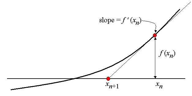
the whole idea is we find the slope `f^'(x)=(y_2-y_1)/(x_2-x_1)`

and the tangent equation finally its roots and this process is repeated until it converges to best possible value at which function has a minimum value.

The Programming language used:PYTHON

CODE:

import matplotlib.pyplot as plt
import numpy as np
from prettytable import PrettyTable as PT

def f(p):	
	#polynomial function value
	return pow(p,3)*c1 + pow(p,2)*c2 + p*c3 - c4

def fprime(p):
	#derivative of the polynommial
	return 3*pow(p,2)*c1 + 2*p*c2 + c3
#initial conditions 
beta=0.5
r=40 #feets
S=150*144 #psi to psf
h=0.6 #feet

#coefficients of the polynomial 
c1=1-pow(beta,2)
c2=0.4*h*pow(beta,2)-(S*pow(h,2)/pow(r,2))
c3=pow(S,2)*pow(h,4)/(3*pow(r,4))
c4=(S*pow(h,2))/(3*pow(r,2))
c4=pow(c4,3)


#plotting the polynomial
func=[]
val=[]
pressure=np.linspace(1,1e8,1000)
for p in pressure:
	#print(p)
	val=f(p)
	#print(val)
	func.append(val)
plt.figure(1)
plt.plot(pressure,func)
plt.xlabel('pressure')
plt.ylabel('function values')
plt.title('Curve for the cushion pressure')
#plt.show()


# CASE 1
#to find out the value of pressure for h = 0.6 ft
alpha=1
p_guess=1000
tol = 1e-4
iter = 1

while (abs(f(p_guess))>tol):

	p_guess=p_guess-(f(p_guess)/fprime(p_guess))*alpha
	iter = iter + 1
		
print('The minumum cushion pressure required for h = 0.6 ft is :',p_guess,'psf')

#CASE 2
#To find the optimal relaxation factor with the help of a plot
alpha=np.linspace(0.1,1.8,10)

num_of_iterations=[]
x=[]
for i in range(0,10):
	
	x=alpha[i]
	p_guess=1000
	tol = 1e-4
	iter = 1

	while (abs(f(p_guess))>tol):

		p_guess=p_guess-(f(p_guess)/fprime(p_guess))*x
		iter = iter + 1
	num_of_iterations.append(iter)
#plotting 
plt.figure(2)
plt.plot(alpha,num_of_iterations,'ro--')
plt.ylabel('num of iterations')
plt.xlabel('relaxation factor alpha')
plt.title('Iterations vs alpha')
print('the optimal relaxation factor(alpha) from the plot is',alpha[-5])
plt.show()

# CASE 3
#Tabulate the results of p for h 
#assuming a suitable relaxation factor
alpha=1.044
#modifying
def f_new(p,h):
	c1=1-pow(beta,2)
	c2=0.4*h*pow(beta,2)-(S*pow(h,2)/pow(r,2))
	c3=pow(S,2)*pow(h,4)/(3*pow(r,4))
	c4=(S*pow(h,2))/(3*pow(r,2))
	c4=pow(c4,3)

	
	#polynomial function value
	return pow(p,3)*c1 + pow(p,2)*c2 + p*c3 - c4

def fprime_new(p,h):
	c1=1-pow(beta,2)
	c2=0.4*h*pow(beta,2)-(S*pow(h,2)/pow(r,2))
	c3=pow(S,2)*pow(h,4)/(3*pow(r,4))
	
	#derivative of the polynommial
	return 3*pow(p,2)*c1 + 2*p*c2 + c3



Thickness = [0.6,1.2,1.8,2.4,3,3.6,4.2] 
Min_Pressure=[]
iter = 1
for h in Thickness:
	p_guess=1000
	tol = 1e-4

	while (abs(f_new(p_guess,h))>tol):
		p_guess=p_guess-(f_new(p_guess,h)/fprime_new(p_guess,h))*alpha
		iter = iter + 1
	Min_Pressure.append(p_guess)
#plotting
plt.figure(3)
plt.plot(Min_Pressure,Thickness,'o-')
plt.xlabel('Min_Pressure')
plt.ylabel('Thickess')
plt.title('Cushion pressure variation with Thickess')
plt.show()
	
#constructing the table
table =PT(['thickness of the ice field(h)','Min cushion pressure (p)'])
for i in range(0,len(Thickness)):
	table.add_row([Thickness[i],Min_Pressure[i]])
print(table)

Explanation to the code:

• after creating a new file with .py extension.
• define the function and its derivatives as of regular form, with coefficients.
• initialize the inputs and compute coefficients from given inputs.
• plot the function takins some values for p to understand the workflow.
• compute the minimum cushion pressure required for h = 0.6 ft by calling the defined functions and using while loop.
• plot the num of iterations vs some values of alpha to find the optimal relaxation factor.
• In the same way, compute min cushion pressure for different thickness values of ice and plot the results.
• draw the table by using PrettyTable.

Results:

The minimum cushion pressure required for h = 0.6 ft is: 4.2390638838316645 psf

the optimal relaxation factor(alpha) from the plot is 1.0444444444444445

+-------------------------------+--------------------------------+
| thickness of the ice field(h) | Min cushion pressure (p) |
+-------------------------------+--------------------------------+
| 0.6 | 4.239062888560484 |
| 1.2 | 17.236690651600195 |
| 1.8 | 38.99008129152081 |
| 2.4 | 69.4992804266107 |
| 3 | 108.76429696183904 |
| 3.6 | 156.78513338234052 |
| 4.2 | 213.56179088298686 |
+-------------------------------+--------------------------------+

Discussion:

• As pressure is a cubic function its curve will be as shown in figure(1).
• Relaxation factor is optimum when it gives the pressure for which function value is minimum with the least number of iterations, in figure(2) alpha[-5] gives the least num of iterations.
• the min cushion pressure required increases with increase in the thickness of the ice which is illustrated in fig(3).

References:

https://brilliant.org/wiki/newton-raphson-method/#:~:text=The%20Newton%2DRaphson%20method%20(also,straight%20line%20tangent%20to%20it.