Genetic Algorithm using MATLAB

AIM: To find the maximum value of the stalagmite function using genetic algorithm.

OBJECTIVES OF THE PROJECT: The objective of this project is to understand the working of the genetic algorithm and make use of it to optimise the given function.

GENETIC ALGORITHM:

Optimization is the process of finding the point that minimizes a function.

The genetic algorithm is a method for solving both constrained and unconstrained optimization problems that are based on natural selection, the process that drives biological evolution.

The genetic algorithm repeatedly modifies a population of individual solutions.

At each step, the genetic algorithm selects individuals at random from the current population to be parents and uses them to produce the children for the next generation. Over successive generations, the population "evolves" toward an optimal solution

• ga uses a set of starting points (called the population) and iteratively generates better points from the population.

The genetic algorithm uses three main types of rules at each step to create the next generation from the current population:

• Selection rules select the individuals, called parents, that contribute to the population at the next generation.
• Crossover rules combine two parents to form children for the next generation.
• Mutation rules apply random changes to individual parents to form children.

GA TERMINOLOGY:

Fitness Functions

The fitness function is the function you want to optimize. For standard optimization algorithms, this is known as the objective function. The toolbox software tries to find the minimum of the fitness function.

Individuals

An individual is any point to which you can apply the fitness function.

An individual is sometimes referred to as a genome and the vector entries of an individual as genes.

Populations and Generations

A population is an array of individuals. For example, if the size of the population is 100 and the number of variables in the fitness function is 3, you represent the population by a 100-by-3 matrix

At each iteration, the genetic algorithm performs a series of computations on the current population to produce a new population. Each successive population is called a new generation.

Diversity

Diversity refers to the average distance between individuals in a population.

A population has high diversity if the average distance is large; otherwise, it has low diversity.

Fitness Values and Best Fitness Values

The fitness value of an individual is the value of the fitness function for that individual. Because the toolbox software finds the minimum of the fitness function, the best fitness value for a population is the smallest fitness value for any individual in the population.

Parents and Children

To create the next generation, the genetic algorithm selects certain individuals in the current population, called parents, and uses them to create individuals in the next generation, called children. Typically, the algorithm is more likely to select parents that have better fitness values.

Working of Genetic Algorithm:

1 The algorithm begins by creating a random initial population.

2 The algorithm then creates a sequence of new populations. At each step, the algorithm uses the individuals in the current generation to create the next population.

To create a new population, the algorithm performs the following steps:

• Scores each member of the current population by computing its fitness value.
• These values are called raw fitness scores.
• Scales the raw fitness scores to convert them into a more usable range of values. These scaled values are called expectation values.
• Selects members, called parents, based on their expectation.
• Some of the individuals in the current population that have lower fitness are chosen as elite. These elite individuals are passed to the next population.
• Produces children from their parents. Children are produced either by making random changes to a single parent—mutation—or by combining the vector entries of a pair of parents—crossover.
• f Replaces the current population with the children to form the next generation.
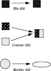
• The genetic algorithm creates three types of children for the next generation:
• Elite are the individuals in the current generation with the best fitness values. These individuals automatically survive to the next generation.
• Crossover is created by combining the vectors of a pair of parents.
• Mutation children are created by introducing random changes, or mutations, to a single parent.
• 

3 The algorithm stops when one of the stopping criteria is met.

Basic Structure of the Genetic Algorithm

The programming language used: MATLAB

stalagmite function:

`f(x,y)=f_(1x)*f_(1y)*f_(2x)*f_(2y)`

`f_(1x)=[sin(5.1*pi*x + 0.5)]^6`

`f_(1y)=[sin(5.1*pi*y + 0.5)]^6`

`f_(2x)=exp^([-4ln(2)*(x-0.0667)^2 /0.64])`

`f_(2y)=exp^([-4ln(2)*(y-0.0667)^2 /0.64])`

code for stalagmite function:

function [Func] = stalagmite(input_vector)
%passing the values of input_vector to x and y.
x = input_vector(1);
y = input_vector(2);

f1=(sin(5.1*pi*x + 0.5)).^6;
f2=(sin(5.1*pi*y + 0.5)).^6;

f3=exp(-4*log(2)*(x-0.0667).^2/(0.64));
f4=exp(-4*log(2)*(y-0.0667).^2/(0.64));
%negative sign is to find the maximum from minumum
Func = -f1*f2*f3*f4;
end

explanation to the code:

• I wrote a function with name stalagmite it takes the input argument(input_vector) and gives out the output argument (func)
• input_vector is necessarily a row vector with two columns so we can extract the values and store them in x & y.
• it computes the value of the function based on the formulae accordingly.

main code:

clear all
close all
clc

%Finding max of Stalagmite function
%defining our search space
x = linspace(0,0.6,150);
y = linspace(0,0.6,150);

num_cases=50;
% preallocation 
f = [];

%creatind 2D arrays using meshgrid
[xx,yy]=meshgrid(x,y);

for i = 1: length(xx)
    
         for j =1: length(yy)
             
              input_vector(1)=xx(i,j);
              input_vector(2)=yy(i,j);
              f(i,j)=stalagmite(input_vector);
         end
         
end
   

% STUDY 1 Unbounded statistical behaviour
tic
for i=1:num_cases
    [inputs, fopt_1(i)]=ga(@stalagmite,2);
    xopt(i)=inputs(1);
    yopt(i)=inputs(2);
end
study_time_1=toc
figure(1)
subplot(2,1,1)

%plotting the stalagmite function with the best fitness value for each iteration 

surfc(xx,yy,-f)
xlabel('x axis')
ylabel('y axis')
zlabel('z axis')
hold on
shading interp
plot3(xopt,yopt,-fopt_1, ...
      'marker','o', ...
      'markerSize',5, ...
      'markerfacecolor','r')
title('unbounded inputs')

subplot(2,1,2)
plot(-fopt_1)
xlabel('iterations')
ylabel('function maximum')



% STUDY 2 bounded statistical behaviour
lb = [0;0]; % Lower bound
ub = [0.8;0.8]; % Upper bound
tic
for i=1:num_cases
    [inputs, fopt_2(i)]=ga(@stalagmite,2,[],[],[],[],lb,ub);
    xopt(i)=inputs(1);
    yopt(i)=inputs(2);
end
study_time_2=toc
figure(2)
subplot(2,1,1)

%plotting the stalagmite function with the best fitness value for each iteration 

surfc(xx,yy,-f)
xlabel('x axis')
ylabel('y axis')
zlabel('z axis')
hold on
shading interp
plot3(xopt,yopt,-fopt_2, ...
      'marker','o', ...
      'markerSize',5, ...
      'markerfacecolor','r')
title('Bounded inputs')

subplot(2,1,2)
plot(-fopt_2)
xlabel('iterations')
ylabel('function maximum')


% STUDY 3 increasing the population
options=optimoptions('ga');
options=optimoptions(options,'populationsize',170);
lb = [0;0]; % Lower bound
ub = [0.8;0.8]; % Upper bound
tic
for i=1:num_cases
    %No linear equality constraints>> You must have Aeq = [] and beq = []
    [inputs, fopt_3(i)]= ...
        ga(@stalagmite,2,[],[],[],[],lb,ub,[],[],options);
    xopt(i)=inputs(1);
    yopt(i)=inputs(2);
end
study_time_3=toc
figure(3)
subplot(2,1,1)

%plotting the stalgmite function with best fittness value for each iteration 
surfc(xx,yy,-f)
xlabel('x axis')
ylabel('y axis')
zlabel('z axis')
hold on
shading interp
plot3(xopt,yopt,-fopt_3, ...
    'marker','o', ...
    'markerSize',5, ...
    'markerfacecolor','r')
title('Increasing population with boudary limits')

subplot(2,1,2)
plot(-fopt_3)
xlabel('iterations')
ylabel('function maximum')


total_study_time=study_time_1 + study_time_2 +study_time_3

results:

for 1st study time

for 2nd study time

for 3rd study time

outputs:

study_time_1 =

9.7577

study_time_2 =

10.6820

study_time_3 =

27.1442

total_study_time =

47.5839

mean(xopt)

ans =

0.0668

>> mean(yopt)

ans =

0.0707

>> mean(-fopt_3)

ans =

0.9969

explanation to the code:

• defining the search space using the linspace command
• using the mesh grid command to generate 2d arrays
• passing these values to stalagmite function as inputs and generate the function.
• study time1:
• we run the GA for multiple number of times using the for loop and the data is stored every time to plot
• the minus sign is taken for the function to find the max using GA, which always finds the min of the function by default.

• Syntax of ga

  To run the genetic algorithm with the default options,

  call ga with the syntax [x,fval] = ga(@fitnessfun, nvars)

  The input arguments to ga are

  • @fitnessfun — A function handle to the file that computes the fitness function.

  The fitness function is the function you want to optimize. For standard optimization algorithms, this is known as the objective function

  • nvars — The number of independent variables for the fitness function.

  The output arguments are

  • x — The final point returned by the algorithm.
  • fval — The value of the fitness function at x
• ga uses the random data so we can not assure that the random samples are close to the search space we defined, in other words, diversity is large.
• study time 2:
• we define the limits so that random data is close to the search space
• syntax

• x = ga(fun,nvars,A,b,Aeq,beq,lb,ub)

  defines a set of lower and upper bounds on the design variables, x, so that a solution is found in the range lb ≤ x ≤ ub.

  Set A=[] and b=[] if no linear inequalities exist.

  Set Aeq=[] and beq=[] if no linear equalities exist.

• the same procedure is followed for the remaining two studies study also
• study time 3:
• ga takes initial population as 50 by default which may not give accurate results as the diversity of the population may be less.
• subplot is used to plot under the same figure.
• syntax:

• x= ga(fun,nvars,A,b,Aeq,beq,lb,ub,nonlcon,options) minimizes with the default optimization parameters replaced by values in options. (Set nonlcon=[] if no nonlinear constraints exist.) Create options using optimoptions

  • fitnessfcn — Fitness function
  • nvars — Number of variables for the problem
  • Aineq — Matrix for inequality constraints
  • Bineq — Vector for inequality constraints
  • Aeq — Matrix for equality constraints
  • Beq — Vector for equality constraints
  • LB — Lower bound on x
  • UB — Upper bound on x
  • nonlcon — Nonlinear constraint function
  • options — Optimization option

Use the debugging tool to correct the errors and to understand the code better.

REFERENCES: https://in.mathworks.com/help/pdf_doc/gads/index.html