Numerical Analysis of Quasi 1-D flow through a Convergent Divergent Nozzle using MacCormack's Technique

Abstract

Numerical analysis of 1-dimensional subsonic supersonic isentropic flow through a converging-diverging nozzle is done using Mac Cormack's technique is done using MATLAB. The numerical study is performed under two methods of formulation i.e., the Conservative form and the Non- Conservative form. The non-dimensional flow properties at the throat of the nozzle are plotted against the number of time steps and the residuals are checked for convergence. The mass flow rate across the non-dimensional nozzle length at steady-state is measured under both conservative and Non-conservative forms and compared with the theoretical value of the mass flow rate. A grid dependence study is performed using two variants of the grid size to compare the accuracy of convergence and the non-dimensional flow properties at steady state.

Introduction

A nozzle is a relatively simple device, just a specially shaped tube through which hot gases flow. Ramjets and rockets typically use a fixed convergent section followed by a fixed divergent section for the design of the nozzle. This nozzle configuration is called a convergent-divergent, or CD, nozzle. In a CD nozzle, the hot exhaust leaves the combustion chamber and converges down to the minimum area, or throat, of the nozzle. The throat size is chosen to choke the flow and set the mass flow rate through the system. The flow in the throat is sonic which means the Mach number is equal to one in the throat. Downstream of the throat, the geometry diverges and the flow is isentropically expanded to a supersonic Mach number that depends on the area ratio of the exit to the throat. The expansion of a supersonic flow causes the static pressure and temperature to decrease from the throat to the exit, so the amount of the expansion also determines the exit pressure and temperature. The exit temperature determines the exit speed of sound, which determines the exit velocity. The exit velocity, pressure, and mass flow through the nozzle determines the amount of thrust produced by the nozzle.

While considering flow through a tube, if the flow is very gradually compressed and then gradually expanded, the flow conditions are restored. So, such a process is a reversible process. According to the Second Law of Thermodynamics, whenever there is a reversible and adiabatic flow, a constant value of entropy is maintained, hence called an isentropic flow of fluids.

Introduction to the Problem

We consider the steady, isentropic flow through a convergent-divergent nozzle as shown below. The flow at the inlet to the nozzle comes from a reservoir where the pressure and temperature are denoted by `p_o` and `T_o` respectively. The cross-sectional area of the reservoir is large, considering `A->oo` theoretically, and hence the velocity is very small i.e., `V->0`. Thus, `p_o` and `T_o` are stagnation values, or total pressure and total temperature respectively. The flow expands isentropically to supersonic speeds at the nozzle exit, where the pressure, temperature, velocity, and Mach number are denoted by `p_e`, `T_e`, `V_e`, and `M_e`. The flow is locally subsonic at the convergent region, sonic at the throat(minimum area), and supersonic at the divergent region. The sonic flow at the throat means that the local velocity at this location is equal to the local speed of sound. Using an asterisk to denote the sonic flow values, we have `V = V^* = a^*`. Similarly, the sonic flow values of pressure and temperature are denoted by `p^*` and `T^*`, respectively. The area of sonic throat is denoted by `A^*`. We assume that at a given section, where the cross sectional area is `A`, the flow properties are uniform across that section. Hence, although the area of the nozzle changes as a function of distance along the nozzle, `x`, and therefore, in reality, the flow field is two dimensional, we make assumptions that the flow properties vary only along with `x`; this is equivalent to assuming uniform flow properties across any given cross section. Such a flow is defined as quasi-one-dimensional flow.

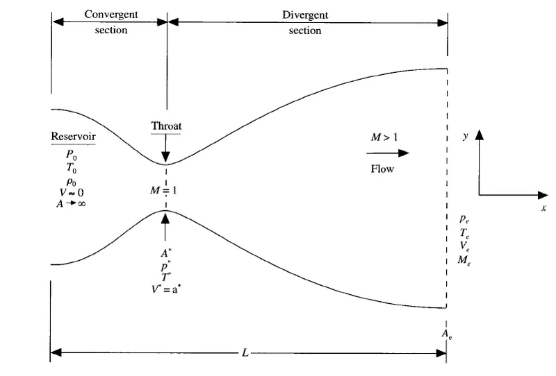
MacCormack's Technique

MacCormack's technique is a variant of Lax-Wendroff's approach but is more simpler in its application. It is an explicit finite-difference technique that is second-order accurate in both space and time. MacCormack's technique is a two step procedure i.e., a predictor and a corrector step. It uses a finite forward difference approach in the predictor step and finite backward difference in the corrector step.

Predictor step

In the first step the solution at the time step `deltat` is predicted using the finite forward difference approach in space to get the time derivative of the non-dimensional property at time `t`.

Corrector step

The second step uses the predicted values of the non-dimensional variables at time `t+deltat` in a finite backward difference approach in space to determine the time derivative of the variable at time `t+deltat`. An average time derivative is obtained by finding the average of the time derivatives at time `t` and `t+deltat` respectively. The averaged time derivative is used to determine the corrected values of the variables at time `t+deltat`.

Determining the time step from Stability criteria

The governing system of equations is hyperbolic with respect to time. A stability constraint exists on this system of equations that is,

`Deltat = C*((Deltax)/(a+V))`

where,

`C` = Courant number

`a` = local speed of sound

`V` = local flow velocity of the fluid

`Deltax` = distance between two consecutive nodes

The simple stability analysis of a linear hyperbolic equation gives the result that `C <= 1` for an explicit numerical solution to be stable. The present application of subsonic-supersonic isentropic nozzle is governed by nonlinear partial differential equations, hence the result `C <= 1` of a linear hyperbolic equation can only be viewed as guidance to the current nonlinear P.D.E. The stability criterion has `a+V` in the denominator which is the Courant-Friedrichs-Lowry(CFL) criterion for a one-dimensional flow.

Convergence criteria

The numerical analysis iterates until the specified number of time steps, but once the solution converges, the time step at which it converges is displayed on the residual visual output. A tolerance of `1xx10^-5` has been set. If the difference between the mass flow rate at time `t+Deltat` and the mass flow rate at time `t` goes below the assigned tolerance value, then the solution is said to have converged.

The Governing flow Equations

Non dimensional Variables

Dimensionless length, `x'` = `x/L`

Temperature, `T'` = `T/(T_o)`

Density, `rho'` = `rho/(rho_o)`

Speed of sound, `a` = `sqrt (T_o)`

Velocity, 'V'' = `V/a`

Area, `A'` = `A/(A^*)`

Time, `t'` = `t/(L/(a_o))`

Since all the parameters in the partial differential equations are non-dimensional, for simplicity, the variables are written in the equation without the `'` symbol.

Non Conservative form

Continuity Equation

`(delrho)/(delt) = -rho((delV)/(delx))-rhoV(delln(A))/(del(x))-V(delrho)/(delx)`

Momentum Equation

`(delV)/(delt) = -V(delT)/(delx)-1/gamma ((delT)/(delx)+T/rho (delrho)/(delx))`

Energy Equation

`(delT)/(delt) = -V(delT)/(delx)-(gamma-1)T[(delV)/(delx)+V (del(lnA))/(delx)]`

Conservative form

Continuity Equation

`(delrhoA)/(delT)+(delrhoAV)/(delx) = 0`

Momentum Equation

`(delrhoAV)/(delt)+(del(rhoAV^2+1/gamma pA))/(delx) = 1/gamma p(delA)/(delx)`

Energy equation

`(del[rho(T/(gamma-1)+gamma/2 V^2)A])/(delt)+(del[rho(T/(gamma-1)+gamma/2 V^2)VA+pAV])/(delx) = 0`

Solution Vectors

`U_1 = rhoA`

`U_2 = rhoAV`

`U_3 = rho(T/(gamma-1)+gamma/2 V^2)A`

Flux Vectors

`F_1 = rhoAV`

`F_2 = rhoAV^2+1/gamma pA`

`F_3 = rho(T/(gamma-1)+gamma/2 V^2)VA+pAV`

The flux terms are represented in terms of primitive variables i.e., `V,T,rho`,and `p`. This makes it difficult for calculations. So, we have expressed the flux vectord in terms of solution venctors, this makes it simpler for calculations.

`F_1 = U_2`

`F_2 = (U_2 ^2)/U_1 + (gamma-1)/gamma (U_3-gamma/2 (U_2 ^2)/U_1)`

`F_3 = gamma (U_2 U_3)/U_1 - gamma(gamma-1)/2 (U_2 ^3)/(U_1 ^2)`

Source term

`J_2 = 1/gamma p (delA)/(delx)`

It can be expressed as a function of solution vectors like this

`J_2 = (gamma-1)/gamma (U_3 - gamma/2 (U_2 ^2)/U_1)(del(lnA))/(delx)`

On substituting the primitive variable with solution, flux ,and source terms the governing equations become

Continuity equation

`(delU_1)/(delt) = -(delF_1)/(delx)`

`(delU_2)/(delt) = -(delF_2)/(delx)+J_2`

`(delU_3)/(delt) = -(delF_3)/(delx)`

Constants and Initial conditions

Length of nozzle = 3m

The specific heat of fluid, `gamma` = 1.4

Assumed Courant number, `C` = 0.5

Tolerance for convergence = `1xx10^-5`

Flow field variables at time `t`=0 are,

1]Non Conservative form

Density, `rho = 1-0.3146x`

Temperature, `T = 1-0.2314x`

Velocity, `V= (0.1+1.09)T^0.5`

2] Conservative form

Density and Temperature

`0<=x<0.5 => {(rho,=,1),(T,=,1):}`

`0.5<=x<1.5 => {(rho,=,1-0.366(x-0.5)),(T,=,1-0.167(x-0.5)):}`

`1.5<=x<3.5 => {(rho,=,0.634-0.3879(x-0.5)),(T,=,0.833-0.3507(x-0.5)):}`

Velocity

`V = 0.59/(rhoA)`

Boundary conditions

Non Conservative form

Subsonic Inlet Boundary Conditons

`rho_1 = 1`

`T_1 = 1`

`V_1 = 2V_2-V_3`

Supersonic Outlet Boundary Conditions

`rho_n = 2rho_(n-1)-rho_(n-2)`

`T_n = 2T_(n-1)-T_(n-2)`

`V_n = 2V_(n-1)-V_(n-2)`

Conservative form

Subsonic Inlet Boundary Conditons

`rho_1 = 1`

`T_1 = 1`

`U_(1_1) = rho_1 A_1`

`U_(2_1) = 2U_(2_2) - U_(2_3)`

`V_1 = (U_(2_1))/(U_(1_1))`

`U_(3_1) = U_(1_1)(T_1/(gamma-1) + gamma/2 V_1^2)`

Supersonic Outlet Boundary Conditions

`U_(1_n) = 2U_(1_(n-1))-U_(1_(n-2))`

`U_(2_n) = 2U_(2_(n-1))-U_(2_(n-2))`

`U_(3_n) = 2U_(3_(n-1))-U_(3_(n-2))`

MATLAB CODE

Main body

close all
clear all
clc

% Initial conditions
n = 61;
gamma = 1.4;
x = linspace(0,3,n);
deltax = x(2)-x(1);
nt = 1400;
A = 1+2.2*(x-1.5).^2;
throat = (n-1)/2+1;
C = 0.5; % Let Courant number be considered as 0.5
rho_ana = 0.634;
M_ana = 1;
P_ana = 0.528;
T_ana = 0.833;

% Non conservative form
[mass_flow_final,rho_nc,V_nc,T_nc,M_nc,P_nc,rho_t_nc,V_t_nc,T_t_nc,M_t_nc,time_nc,P_t_nc] = non_cons_form(n,x,deltax,throat,gamma,nt,A,C,rho_ana,M_ana,P_ana,T_ana);

% Conservative form
[u1,u2,u3,mass_flow_c_final,rho,V,T,M,P,rho_t,V_t,T_t,M_t,time_c,P_t] = conservative_form(n,x,deltax,throat,gamma,nt,A,C,rho_ana,M_ana,P_ana,T_ana);

for y = 1:n
    analytical_massflow(y) = 0.579;
end

figure(7),clf
hold on;
plot(x,mass_flow_final,'-','color',[.1 .7 .3],'linew',2);
plot(x,mass_flow_c_final,'-','color',[0.4 0.3 0.7],'linew',2);
plot(x,analytical_massflow,'--b','linew',2);
xlabel('Nozzle nodes');
ylabel('Mass flow rate(Non Dimensional)');
title({'Theoreitcal and Analytical mass flow rates'});
legend('Non Conservative form','Conservative form','Experimental value');

Function of the Non Conservative Form

function [mass_flow_final,rho_nc,V_nc,T_nc,M_nc,P_nc,rho_t_nc,V_t_nc,T_t_nc,M_t_nc,time_nc,P_t_nc] = non_cons_form(n,x,deltax,throat,gamma,nt,A,C,rho_ana,M_ana,P_ana,T_ana)
tic
% Initial conditions
rho_nc = 1-0.3146*x;
T_nc = 1-0.2314*x;
V_nc = (0.1+1.09*x).*T_nc.^0.5;

rho_t_nc = zeros(1,nt);
T_t_nc = zeros(1,nt);
V_t_nc = zeros(1,nt);
M_t_nc = zeros(1,nt);
P_t_nc = zeros(1,nt);
error_ncm = zeros(1,nt);

tol = 1e-5;

drhocdt_res = zeros(1,nt);
dVcdt_res = zeros(1,nt);
dTcdt_res = zeros(1,nt);

for t_s = 1:nt
    
    rho = rho_nc;
    T = T_nc;
    V = V_nc;
    mass_f_o = rho.*V.*A;
    % Predictor step
    
    % Finding the minimum time step
    a = T.^0.5;
    dt = (C*deltax)./(a+V);
    dt = min(dt);
    
    drhodt = zeros(1,n);
    dVdt = zeros(1,n);
    dTdt = zeros(1,n);
    rhop = zeros(1,n);
    Vp = zeros(1,n);
    Tp = zeros(1,n);
    
    % At time t
    for i = 2:n-1
        drhodt(i) = -rho(i)*(V(i+1)-V(i))/deltax - rho(i)*V(i)*(log(A(i+1))-log(A(i)))/deltax - V(i)*(rho(i+1)-rho(i))/deltax;
        dVdt(i) = -V(i)*(V(i+1)-V(i))/deltax - ((T(i+1)-T(i))/deltax + (T(i)/rho(i))*(rho(i+1)-rho(i))/deltax)/gamma;
        dTdt(i) = -V(i)*(T(i+1)-T(i))/deltax - (gamma-1)*T(i)*(V(i)*(log(A(i+1))-log(A(i)))/deltax + (V(i+1)-V(i))/deltax);
        
        % At time t+dt
        rhop(i) = rho(i)+dt*drhodt(i);
        Vp(i) = V(i)+dt*dVdt(i);
        Tp(i) = T(i)+dt*dTdt(i);
    end
    
    % 1st node of predicted value
    
    rhop(1) = 1;
    Tp(1) = 1;
    Vp(1) = 2*Vp(2)-Vp(3);
    
    % Last node of predicted value
    
    Vp(n) = 2*Vp(n-1) - Vp(n-2);
    Tp(n) = 2*Tp(n-1) - Tp(n-2);
    rhop(n) = 2*rhop(n-1) - rhop(n-2);
    
    % Corrector step%
    
    drhopdt = zeros(1,n);
    dVpdt = zeros(1,n);
    dTpdt = zeros(1,n);
    drhocdt = zeros(1,n);
    dVcdt = zeros(1,n);
    dTcdt = zeros(1,n);
    
    % At time t+dt
    for j = 2:n-1
        drhopdt(j) = -rhop(j)*(Vp(j)-Vp(j-1))/deltax - (rhop(j))*(Vp(j))*((log(A(j))-log(A(j-1)))/deltax)-Vp(j)*(rhop(j)-rhop(j-1))/deltax;
        dVpdt(j) = -Vp(j)*(Vp(j)-Vp(j-1))/deltax - ((Tp(j)-Tp(j-1))/deltax + (Tp(j)/rhop(j))*(rhop(j)-rhop(j-1))/deltax)/gamma;
        dTpdt(j) = -Vp(j)*(Tp(j)-Tp(j-1))/deltax - (gamma-1)*Tp(j)*((Vp(j)-Vp(j-1))/deltax + Vp(j)*(log(A(j))-log(A(j-1)))/deltax);
        
        % Corrected derivative i.e., average of derivatives
        
        drhocdt(j) = 0.5*(drhodt(j)+drhopdt(j));
        dVcdt(j) = 0.5*(dVdt(j)+dVpdt(j));
        dTcdt(j) = 0.5*(dTdt(j)+dTpdt(j));
        
        % Corrected values at t+dt
        rho_nc(j) = rho(j) + dt*drhocdt(j);
        V_nc(j) = V(j) + dt*dVcdt(j);
        T_nc(j) = T(j) + dt*dTcdt(j);
        
    end
    
    % 1st node of corrected value
    
    rho_nc(1) = 1;
    T_nc(1) = 1;
    V_nc(1) = 2*V_nc(2)-V_nc(3);
    
    % Last node of corrected value
    
    V_nc(n) = 2*V_nc(n-1) - V_nc(n-2);
    T_nc(n) = 2*T_nc(n-1) - T_nc(n-2);
    rho_nc(n) = 2*rho_nc(n-1) - rho_nc(n-2);
    
    %Pressure ratio
    P_nc = rho_nc.*T_nc;
    % mach number
    M_nc = V_nc./(T_nc.^0.5);
    % Mass flow rate
    mass_flow_nc = rho_nc.*V_nc.*A;
    
    % Convergence
    error_ncm(t_s) = max(abs(mass_f_o-mass_flow_nc));
    
    % Residuals
    drhocdt_res(t_s) = abs(drhocdt(throat));
    dTcdt_res(t_s) = abs(dTcdt(throat));
    dVcdt_res(t_s) = abs(dVcdt(throat));
    
    % At throat
    rho_t_nc(t_s) = rho_nc(throat);
    T_t_nc(t_s) = T_nc(throat);
    V_t_nc(t_s) = V_nc(throat);
    M_t_nc(t_s) = M_nc(throat);
    P_t_nc(t_s) = P_nc(throat);
    
    hold on;
    figure(2)
    if t_s == 1
        plot(x,mass_flow_nc,'--','color',[.1 .5 .9],'linew',0.5);
    elseif t_s == 50
        plot(x,mass_flow_nc,'-','color',[.2 .2 .8],'linew',1);
    elseif t_s == 100
        plot(x,mass_flow_nc,'-','color',[.3 .4 .7],'linew',1);
    elseif t_s == 150
        plot(x,mass_flow_nc,'-','color',[.4 .9 .6],'linew',1);
    elseif t_s == 200
        plot(x,mass_flow_nc,'-','color',[.5 .1 .5],'linew',1);
    elseif t_s == 700
        plot(x,mass_flow_nc,'-','color',[.6 .3 .4],'linew',1);
    elseif t_s == 1400
        plot(x,mass_flow_nc,'-','color',[.7 .5 .3],'linew',1);
        xlabel('Distance through nozzle(x) - (Non Dimensional)');
        ylabel('Mass flow rate(Non dimensional)');
        grid minor;
        legend('1deltat','50deltat','100deltat','150 deltat','200 deltat','700 deltat','1400deltat');
        title({'Non Conservative form';'Instantaneous mass flow rates at different time steps'});
    end
    
end

% At steady state
mass_flow_final = mass_flow_nc;

% Finding convergence point
for i=1:nt
    if error_ncm(i)<tol
        mar = i;
        break;
    end
end    

time_nc = toc;

% Residuals and convergence point
figure(8)
hold on;
plot(1:nt,drhocdt_res,'color',[0.1 0.2 0.3],'linew',2);
plot(1:nt,dTcdt_res,'color',[0.4 0.2 0.7],'linew',2);
plot(1:nt,dVcdt_res,'color',[0.8 0.5 0.3],'linew',2);

Ylow = min([drhocdt_res dTcdt_res dVcdt_res])-0.1*abs(max([drhocdt_res dTcdt_res dVcdt_res]));
Yhigh = max([drhocdt_res dTcdt_res dVcdt_res])+0.1*abs(max([drhocdt_res dTcdt_res dVcdt_res]));
ylim([Ylow Yhigh]);

plot([mar mar],get(gca,'Ylim'),'-r');
text(mar-30,max([drhocdt_res dTcdt_res dVcdt_res])/3,strcat('Convergence time = ',num2str(mar),' \deltat'),'Rotation',90,'FontSize',8)

title({'Scaled Residuals'});
xlabel('Time');
ylabel('Residuals');
% Properties at the throat varying with time
figure(1)

subplot(4,1,1)
hold on;
plot(1:nt,P_t_nc,'linew',2);
plot(1:nt,P_ana*ones(1,1400),'--r','linew',0.5);
xlabel('No. of time steps');
ylabel('Pressure');
title({'Variables at nozzle throat with timestep'});
legend('Analytical','Theoretical');

subplot(4,1,2)
hold on;
plot(1:nt,T_t_nc,'linew',2);
plot(1:nt,T_ana*ones(1,1400),'--r','linew',0.5);
xlabel('No. of time steps');
ylabel('Temperature');
legend('Analytical','Theoretical');

subplot(4,1,3)
hold on;
plot(1:nt,rho_t_nc,'linew',2);
plot(1:nt,rho_ana*ones(1,1400),'--r','linew',0.5);
xlabel('No. of time steps');
ylabel('Density');
legend('Analytical','Theoretical');

subplot(4,1,4)
hold on;
plot(1:nt,M_t_nc,'linew',2);
plot(1:nt,M_ana*ones(1,1400),'--r','linew',0.5);
xlabel('No. of time steps');
ylabel('Mach number');
legend('Analytical','Theoretical');

% Properties along the non dimensional nozzle length at steady state
figure(3),clf
subplot(411)
plot(x,rho_nc,'linew',2);
ylabel('rho/rho_o');
title('Variables at steady state using Non-conservative form');

subplot(412)
plot(x,T_nc,'linew',2);
ylabel('T/T_o');

subplot(413)
plot(x,P_nc,'linew',2);
ylabel('P/P_o');

subplot(414)
plot(x,M_nc,'linew',2);
ylabel('Mach number(M)');

Function of the Conservative Form

function [u1,u2,u3,mass_flow_c_final,rho,V,T,M,P,rho_t,V_t,T_t,M_t,time_c,P_t] = conservative_form(n,x,deltax,throat,gamma,nt,A,C,rho_ana,M_ana,P_ana,T_ana)
% calculating initial profiles
tic

error_c = zeros(1,nt);
rho = zeros(1,n);
T = zeros(1,n);
V = zeros(1,n);
for i=1:n
    if x(i)>=0 && x(i)<0.5
        rho(i) = 1;
        T(i) = 1;
        %V(i) = (0.1 + 1.09*x(i)).*T(i).^0.5;
    elseif x(i)>=0.5 && x(i)<1.5
        rho(i) = 1 - 0.366*(x(i)-0.5);
        T(i) = 1 - 0.167*(x(i)-0.5);
        %V(i) = (0.1 + 1.09*x(i)).*T(i).^0.5;
    elseif x(i)>=1.5 && x(i)<=3.5
        rho(i) = 0.634 - 0.3879*(x(i)-1.5);
        T(i) = 0.833 - 0.3507*(x(i)-1.5);
        %V(i) = (0.1 + x(i)).*T(i).^0.3;
    end
end

% Steady flow is assumed for initial condition
V = 0.59./(rho.*A);

tol = 1e-5;

% Solution vectors
u1 = rho.*A;
u2 = rho.*A.*V;
u3 = rho.*(T./(gamma-1)+(gamma/2)*V.^2).*A;
P = rho.*T;% Non dimensional Pressure

rho_t = zeros(1,nt);
T_t = zeros(1,nt);
P_t = zeros(1,nt);
V_t = zeros(1,nt);
M_t = zeros(1,nt);

du1dt_res = zeros(1,nt);
du2dt_res = zeros(1,nt);
du3dt_res = zeros(1,nt);

for k = 1:nt
    % Updating old values
    u1_o = u1;
    u2_o = u2;
    u3_o = u3;
    mass_flow_co = rho.*V.*A;
    
    %time step
    a = T.^0.5;
    dt = (C*deltax)./(a+V);
    dt = min(dt);
    
    % Flux terms
    f1 = u2_o;
    f2 = ((u2_o.^2)./u1_o)+((gamma-1)/gamma)*(u3_o - (gamma/2)*(u2_o.^2)./u1_o);
    f3 = ((gamma*u2_o.*u3_o)./u1_o)-(gamma*(gamma-1)/2)*(u2_o.^3./(u1_o.^2));
    
    % Predictor step
    
    j2 = zeros(1,n);
    du1pdt = zeros(1,n);
    du2pdt = zeros(1,n);
    du3pdt = zeros(1,n);
    
    
    for j=2:n-1
        % Source term
        j1(j) = (1/gamma)*rho(j).*T(j).*((A(j+1)-A(j))/deltax);
        
        %Continuity equation
        du1pdt(j) = -(f1(j+1)-f1(j))/deltax;
        
        % Momentum equation
        du2pdt(j) = -(f2(j+1)-f2(j))/deltax + j1(j);
        
        %Energy equation
        du3pdt(j) = -(f3(j+1)-f3(j))/deltax;
        
        % Predited values
        u1(j) = u1_o(j)+dt*du1pdt(j);
        u2(j) = u2_o(j)+dt*du2pdt(j);
        u3(j) = u3_o(j)+dt*du3pdt(j);
        
    end
    
    % Predicted values of primitive variables
    rhop = u1./A;
    Vp = u2./u1;
    Tp = (gamma-1)*(u3./u1 - (gamma/2)*(Vp.^2));
    
    % Updating flux terms from u1 u2 u3 values
    f1 = u2;
    f2 = ((u2.^2)./u1)+((gamma-1)/gamma)*(u3 - (gamma/2)*(u2.^2)./(u1));
    f3 = ((gamma*u2.*u3)./u1)-(gamma*(gamma-1)/2)*(u2.^3./(u1.^2));
    
    % Corrector step
    
    du1cdt = zeros(1,n);
    du2cdt = zeros(1,n);
    du3cdt = zeros(1,n);
    du1dt = zeros(1,n);
    du2dt = zeros(1,n);
    du3dt = zeros(1,n);
    
    for j=2:n-1
        % Source term
        j2(j) = (1/gamma)*rhop(j).*Tp(j).*((A(j)-A(j-1))/deltax);
        
        %Continuity equation
        du1cdt(j) = -(f1(j)-f1(j-1))/deltax;
        
        % Momentum equation
        du2cdt(j) = -(f2(j)-f2(j-1))/deltax + j2(j);
        
        %Energy equation
        du3cdt(j) = -(f3(j)-f3(j-1))/deltax;
        
        % Compute average time derivative
        du1dt(j) = 0.5*(du1pdt(j)+du1cdt(j));
        du2dt(j) = 0.5*(du2pdt(j)+du2cdt(j));
        du3dt(j) = 0.5*(du3pdt(j)+du3cdt(j));
    end
    
    
    % final solution update
    for i=2:n-1
        u1(i) = u1_o(i)+du1dt(i)*dt;
        u2(i) = u2_o(i)+du2dt(i)*dt;
        u3(i) = u3_o(i)+du3dt(i)*dt;
    end
    
    % Applying boundary conditions
    
    % Inlet boundary
    rho(1) = 1;
    T(1) = 1;
    
    u1(1) = rho(1)*A(1);
    u2(1) = 2*u2(2)-u2(3);
    % Intermediate variable
    V(1) = u2(1)/u1(1);
    
    u3(1) = u1(1)*(T(1)/(gamma-1))+(gamma/2)*(V(1)^2);
    
    % Outlet boundary conditions
    u1(n) = 2*u1(n-1)-u1(n-2);
    u2(n) = 2*u2(n-1)-u2(n-2);
    u3(n) = 2*u3(n-1)-u3(n-2);
    
    % Corrected values of primitive variables
    rho = u1./A;
    V = u2./u1;
    T = (gamma-1)*(u3./u1 - (gamma/2)*(V.^2));
    
    % Solutions
    M = V./(T.^0.5);
    P = rho.*T;
    mass_flow_com = rho.*V.*A;
    
    % Convergence
    error_c(k) = max(abs(mass_flow_co-mass_flow_com));
    
    du1dt_res(k) = du1dt(throat);
    du2dt_res(k) = du2dt(throat);
    du3dt_res(k) = du3dt(throat);
    
    % At throat
    rho_t(k) = rho(throat);
    T_t(k) = T(throat);
    P_t(k) = P(throat);
    V_t(k) = V(throat);
    M_t(k) = M(throat);
    
    figure(4)
    hold on;
    if k == 1
        plot(x,mass_flow_com,'--','color',[.1 .5 .9],'linew',0.5);
    elseif k == 50
        plot(x,mass_flow_com,'-','color',[.2 .4 .8]','linew',1);
    elseif k == 100
        plot(x,mass_flow_com,'-','color',[.3 .6 .7],'linew',1);
    elseif k == 150
        plot(x,mass_flow_com,'-','color',[.4 .9 .6],'linew',1);
    elseif k == 200
        plot(x,mass_flow_com,'-','color',[.5 .2 .5],'linew',1);
    elseif k == 700
        plot(x,mass_flow_com,'-','color',[.6 .1 .4],'linew',1);
    elseif k == 1400
        plot(x,mass_flow_com,'-','color',[.7 .1 .3],'linew',1);
        xlabel('Distance through nozzle(x) - (Non Dimensional)');
        ylabel('Mass flow rate(Non dimensional)');
        grid minor;
        legend('1deltat','50deltat','100deltat','150 deltat','200 deltat','700 deltat','1400 deltat');
        title({'Conservative form';'Instantaneous mass flow rates at different time steps'});
    end
    
    
    
end

mass_flow_c_final = mass_flow_com;

% Finding convergence point
for i=1:nt
    if error_c(i)<tol
        res = i;
        break;
    end
end

time_c = toc;

% Residuals and convergence point
figure(9)
hold on;
plot(1:nt,du1dt_res,'color',[0.2 0.7 0.5],'linew',2);
plot(1:nt,du2dt_res,'color',[0.5 0.3 0.9],'linew',2);
plot(1:nt,du3dt_res,'color',[0.8 0.6 0.2],'linew',2);

ylow = min([du1dt_res du2dt_res du3dt_res])-0.1*abs(max([du1dt_res du2dt_res du3dt_res]));
yhigh = max([du1dt_res du2dt_res du3dt_res])+0.1*abs(max([du1dt_res du2dt_res du3dt_res]));
ylim([ylow yhigh]);

plot([res res],get(gca,'Ylim'),'-r');
text(res-30,max([du1dt_res du2dt_res du3dt_res])/5,strcat('Convergence time = ',num2str(res),' \deltat'),'Rotation',90,'FontSize',8)

title({'Scaled Residuals'});
xlabel('Time');
ylabel('Residuals');

% Properties at the throat varying with time

figure(5)
subplot(4,1,1)
hold on;
plot(1:nt,P_t,'linew',2);
plot(1:nt,P_ana*ones(1,1400),'--r','linew',0.5);
xlabel('No. of time steps');
ylabel('Pressure');
title({'Variables at nozzle throat with timestep'});
legend('Analytical','Theoretical');

subplot(4,1,2)
hold on;
plot(1:nt,T_t,'linew',2);
xlabel('No. of time steps');
plot(1:nt,T_ana*ones(1,1400),'--r','linew',0.5);
ylabel('Temperature');
legend('Analytical','Theoretical');

subplot(4,1,3)
hold on;
plot(1:nt,rho_t,'linew',2);
plot(1:nt,rho_ana*ones(1,1400),'--r','linew',0.5);
xlabel('No. of time steps');
ylabel('Density');
legend('Analytical','Theoretical');

subplot(4,1,4)
hold on;
plot(1:nt,M_t,'linew',2);
plot(1:nt,M_ana*ones(1,1400),'--r','linew',0.5);
xlabel('No. of time steps');
ylabel('Mach number');
legend('Analytical','Theoretical');

% Properties along the non dimensional nozzle length at steady state
figure(6),clf
subplot(411)
plot(x,rho,'linew',2);
ylabel('rho/rho_o');
title('Variables at steady state using Conservative form');

subplot(412)
plot(x,T,'linew',2);
ylabel('T/T_o');

subplot(413)
plot(x,P,'linew',2);
ylabel('P/P_o');

subplot(414)
plot(x,M,'linew',2);
ylabel('Mach number(M)');

RESULTS

The below obtained results have been derived by discretizing the non dimensional 1-D nozzle into 31 nodes.

Non Conservative form

1)Scaled Residuals

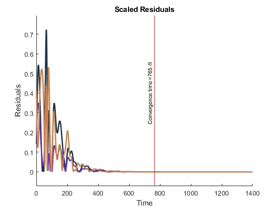
The Non conservative form of the equations were iterated for 1400 time steps and they have converged at the 765th time step. In the time steps beyond the 765th time step, the flow through the nozzle has attained steady state.

2) Mass Flow rate along the non dimensional length of the nozzle at different time steps.

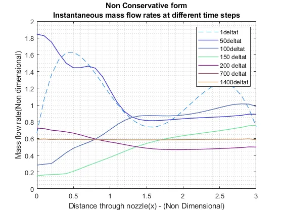
This depicts mass flow rates along the non dimensional length of the nozzle at different time steps. At the 1400th time step the mass flow rate has converged to a single value.

3) Variation of the dependent variables with time

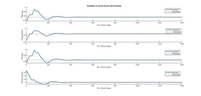
The above plot shows the variables converge with the theoretical value along time when solved in the non conservative form. The analytical and predicted values of the variables appear to be very close in the plot.

4)Variables along the non dimensional length of the nozzle under steady state

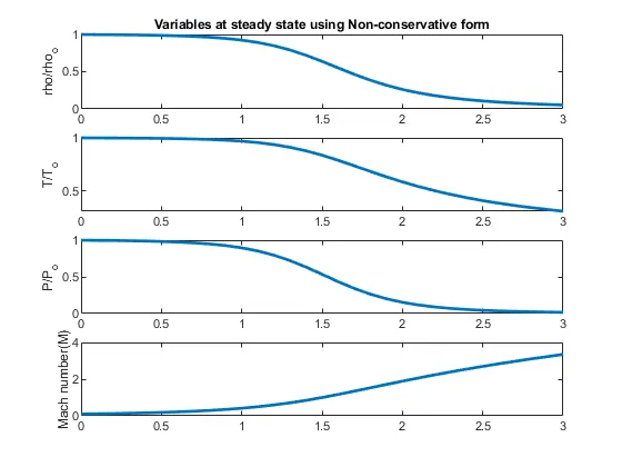
The variables have a smooth transition from the subsonic region to the supersonic region of the nozzle.

Conservative form

1) Scaled Residuals

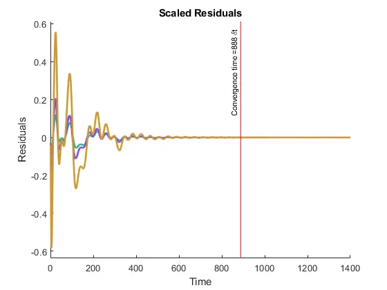
The Conservative form of the equations were iterated for 1400 time steps and they have converged at the 888th time step. The residuals of the conservative form is observed to oscillate between positive and negative values and finally converge near zero. In the time steps beyond the 888th time step, the flow through the nozzle has attained steady state.

2) Mass Flow rate along the non dimensional length of the nozzle at different time steps.

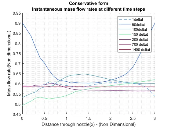
This depicts mass flow rates along the non dimensional length of the nozzle at different time steps. At the 1400th time step the mass flow rate has converged to a single value. When compared with the converged line in the Non conservative form, this line seems to be below the former.

3) Variation of the dependent variables with time

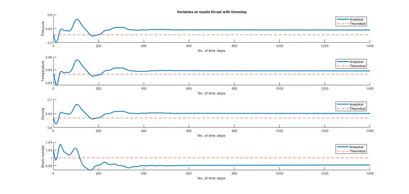
The above plot shows the variables converge parallel to the theoretical value along time when solved in the conservative form. The analytical and predicted values of the variables appear to have some offset in the steady state.

4)Variables along the non dimensional length of the nozzle under steady state

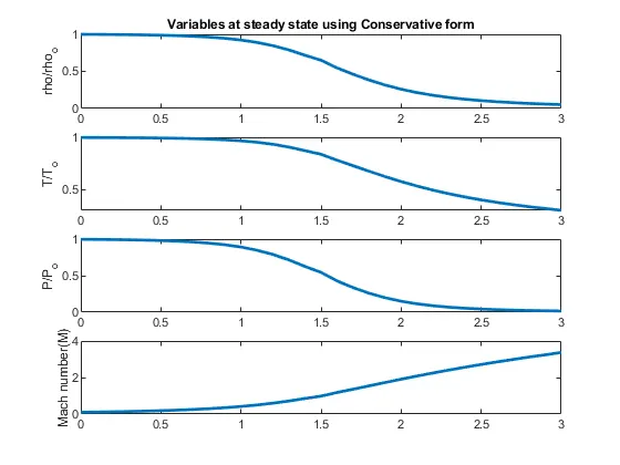
The variables have a smooth transition from the subsonic region to the supersonic region of the nozzle.

Comparision of Mass flow rates obtained by the Conservative form and the Non Conservative form with the Theoretical value

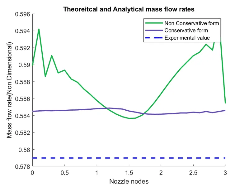
The mass flow rate distribution obtained by the Non-Conservative form has a very irregular distribution along the non-dimensional length of the nozzle. The mass flow rate distribution obtained by the conservative form has a very uniform distribution along the length of the nozzle closely parallel to the theoretical mass flow.

Grid Dependency Test

Grid dependency test is performed to evaluate the dependency of the accuracy of the obtained results on the number of nodes used to descretize the model. The above results were obtained by using 31 nodes along the non dimensional length of the nozzle. By replacing the value assigned to the variable representing the number of nodes by 61, another numerical analysis has been conducted.

The below obtained results have been derived by discretizing the non dimensional 1-D nozzle into 61 nodes.

Non Conservative form

1)Scaled Residuals

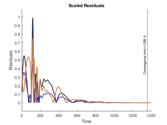
The Non conservative form of the equations were iterated for 1400 time steps and they have converged at the 1359th time step. The residuals seem to vary by values greater than the tolerance value for many time steps. In the few time steps beyond the 1359th time step, the flow through the nozzle has attained steady state.

Conservative form

1)Scaled Residuals

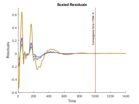
The Conservative form of the equations were iterated for 1400 time steps and they have converged at the 1004th time step. The residuals of the conservative form is observed to oscillate between positive and negative values and finally converge near zero. In the time steps beyond the 1004th time step, the flow through the nozzle has attained steady state.

The below table shows the dependence of either form of governing equations on the number of nodes along the non dimensional length of the nozzle.

Cases	Number of nodes	Density	Temperature	Pressure	Mach number
Non Conservative form	31	0.6386	0.8364	0.5341	0.9994
Non Conservative form	61	0.6375	0.8354	0.5326	0.9997
Conservative form	31	0.6504	0.8381	0.5451	0.9817
Conservative form	61	0.6382	0.8332	0.5318	0.9994
Theoretical values		0.634	0.833	0.528	1

1. There is a good improvement in the accuracy of the conservative form, but the accuracy of the non conservative form has improved only by a small margin.
2. On increasing the number of nodes a few variables have become accurate from the Conservative form, while the rest have become accurate from the Non conservative form.

The below table shows the time taken for both the forms of the governing equations to complete the calculation of variables using MacCormack's technique and the number of time steps for the equations to converge.

Case	Number of nodes	Completion time(seconds)	Time steps for Convergence
Non Conservative form	31	3.6548	765
Non Conservative form	61	3.6223	1359
Conservative form	31	3.2626	888
Conservative form	61	3.3581	1004

1. The Conservative form has finished the calculation of variables earlier than the Non-conservative form under both the grid conditions.
2. The Non Conservative form achieved convergence in fewer time steps than the Conservative form when 31 nodes were used. But the Conservative form achieved convergence in fewer time steps when 61 nodes were used.

CONCLUSIONS

1. There is no superiority in either form of governing equations when accuracy is considered. Both forms give a good degree of accuracy.
2. The mass flow distribution is better in the Conservative form, it does a good job in conserving mass.
3. The residuals of the Conservative form oscillate in between positive and negative values before reaching stability, but residuals of the Non Conservative form remain positive.
4. The results are obtained faster from the Conservative form in its case.
5. Both the forms of governing equations gave satisfactory results.
6. The solution can be said to be grid independent.
7. Considering C`<=`1 for the current non linear application turned out beneficial in obtaining grid independent solutions.
8. Based on the current study, Non Conservative form has better accuracy when there are less number of nodes and Conservative form has better accuracy when there are more nodes.