Python Program: Newton-Raphson Iterator to Determine Min. Pressure
Aim: Determining minimum pressure to break ice using an air cushion vehicle
Objective:
- Finding minimum pressure for different thickness of ice sheets using Newton Raphson method.
- Finding a suitable relaxation factor at h = 0.6 ft.
- Tabulating and plotting the results.
Theory:
Newton Raphson Method:
In numerical analysis, Newton-Raphson method (NR method), is a root finding algorithm which produces successively better approximations to the roots (or zeroes) of a real valued function. The most basic version starts with a single variable function `f` defined for a real variable `x`, the function's derivative `f'`, and an initial guess `x0` for a root of `f`. If the function satisfies sufficient assumptions and the intitial guess is close, then
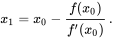
The iterative form is given as
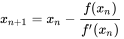
Air Cushion Vehicle:
The function is provided to us, which has to be minimised to determine pressure required to break ice of given thickness.
where,
p = cushion pressure
h = thickness of ice field
r = size of air cushion
`sigma` = tensile strength of ice`
`beta` = width of ice wedge
Program:
Part-1: Minimum pressure for various thickness
#Importing Required Libraries
from numpy import *
from matplotlib.pyplot import *

#Inputs
b = 0.5 							#Beta
r = 40  							#Size of Air Cushion in feet
s = 150*144 						#sigma: tensile strength of Ice in psi (converted to pound per square foot by multiplying 144)
h = [0.6,1.2,1.8,2.4,3.0,3.6,4.2] 	# Multiple thickness of Ice field given in Feet (the multiple values are clubbed in an array for ease)
tol = 1e-5	                        #Considering the convergence criteria for the pressure equation
i = 1
p_guess = 100						#Providing an initial guess value for pressure


#Defining the pressure equation for Air Cushion Vehicle
def f(p,h):
	return ((pow(p,3)*(1-pow(b,2)))+ ((0.4*h*pow(b,2) - (s*pow(h,2)/pow(r,2)))*pow(p,2)) + (pow(s,2)*pow(h,4)*p/(3*pow(r,4))) - (pow((s*pow(h,2)/(3*pow(r,2))),3)))

#Defining the 1st order derivative (w.r.t pressure) function of the equation
def f_prime(p,h):
	return ((3*pow(p,2)*(1-pow(b,2)))+ 2*p*(0.4*h*pow(b,2) - (s*pow(h,2)/pow(r,2)))+ (pow(s,2)*pow(h,4)/(3*pow(r,4))))

#Defining Pressure and Iteration Array
min_pressure = []
iter = []

#Loop to calculate minimum pressure for various ice sheet thickness
for x in h:
	alpha = 1
	i=1
	 #Using an exit controlled loop which would terminate when the convergence criteria is met by performing Newton Raphson method
	while(abs(f(p_guess,x))>tol):
		p_guess = p_guess - alpha * (f(p_guess,x)/f_prime(p_guess,x))
		i=i+1

	p_guess = round(p_guess/144, 8)
	iter.append(i)
	min_pressure.append(p_guess)
	p_guess=100

#Printing the results in a tabular format
print("---------------------------------------------------------------------------------------------")
for j in range(0,len(h)):
	if j == 0:
		print('| Ice Thickness (feet) |', 'Min. Air Cushion Pressure (psi) |', 'No. of Iteration for Convergence |')
	print("---------------------------------------------------------------------------------------------")
	print('|     ', h[j], '            |          ', min_pressure[j], '           |              ', iter[j],'                |')
print("---------------------------------------------------------------------------------------------")

#Plotting
plot(h,min_pressure)
xlabel('Ice Field Thickness (feet)')
ylabel('Min. Air Cushion Pressure (psi)')
title('Air Cushion Pressure vs Ice Field Thickness')
savefig("airpressure-icethickness.png")
show()
1. The program starts with importing the required libraries. We need numpy for calculations and matplotlib.pyplot for plotting graphs.
2. The specified inputs are given, keeping in mind that the units are kept consistent. Further, we need to define the pressure equation as a function in python which takes in pressure and height values and return the solution. Similarly, we define the first order derivative of the function which we'll use in NR method iterations. Later, we define empty array of minimum pressure and iterations.
3. To code Newton-Raphson, we need to iterate a block of code. This is done by using for loop. The tolerance value (provided in input) helps to make an exit condition and to ensure that the iterator exits on passing of the minimum value. This exit condition is used in while loop.
4. Thus, the function called in the aforementioned loops gives minimum pressure values and number of iterations are counted using loop counter. This is appended in the empty arrays created previously using append command. A for loop helps in printing the results in tabular fashion (using print command) and plots are embelished with suitable labels and titles.
Output:
Part-2: Optimum value of relaxation factor (alpha) for h=0.6ft
#Importing Required Libraries
from matplotlib.pyplot import *
from numpy import *

#Inputs
b = 0.5 							#Beta
r = 40  							#Size of Air Cushion in feet
s = 150*144 						#sigma: tensile strength of Ice in psi (converted to pound per square foot by multiplying 144)
h = 0.6							 	# Multiple thickness of Ice field given in Feet (the multiple values are clubbed in an array for ease)
tol = 1e-5	                        #Considering the convergence criteria for the pressure equation


def f(p):
	return ((pow(p,3)*(1-pow(b,2)))+ ((0.4*h*pow(b,2) - (s*pow(h,2)/pow(r,2)))*pow(p,2)) + (pow(s,2)*pow(h,4)*p/(3*pow(r,4))) - (pow((s*pow(h,2)/(3*pow(r,2))),3)))

#Defining the 1st order derivative (w.r.t pressure) function of the equation
def df(p):
	return ((3*pow(p,2)*(1-pow(b,2)))+ 2*p*(0.4*h*pow(b,2) - (s*pow(h,2)/pow(r,2)))+ (pow(s,2)*pow(h,4)/(3*pow(r,4))))


a = linspace(0.1,1.9,20)
pressure = []
count = []
p_guess = 100
for x in a:
	i=1
	#Using an exit controlled loop which would terminate when the convergence criteria is met by performing Newton Raphson method
	while(abs(f(p_guess))>tol):
		p_guess = p_guess - x * (f(p_guess)/df(p_guess))
		i=i+1
	pressure.append(p_guess)
	p_guess = 100
	count.append(i)

#Plotting
figure(1)
plot(a,count)
xlabel('Alpha')
ylabel('No. of Interations')
title('Iterations vs Alpha')
savefig("alpha-iterations.png")
show()

figure(2)
plot(a,pressure)
xlabel('Alpha')
ylabel('Pressure (psi)')
title('Pressure vs Alpha')
savefig("alpha-pressure.png")
show()
1. The program starts with importing the required libraries. We need numpy for calculations and matplotlib.pyplot for plotting graphs.
2. The specified inputs are given, keeping in mind that the units are kept consistent. Further, we need to define the pressure equation as a function in python which takes in pressure and height values and return the solution. Similarly, we define the first order derivative of the function which we'll use in NR method iterations.
3. We define an array of alpha values to find an optimum value among them. Also empty array of pressure and iterations are created.
4. To code Newton-Raphson, we need to iterate a block of code. This is done by using for loop. The tolerance value (provided in input) helps to make an exit condition and to ensure that the iterator exits on passing of the minimum value. This exit condition is used in while loop. The outputs are appended into the empty arrays.
5. As, we have two plots, we use figure command to get two separate plot windows. The plots are of alpha vs iterations and alpha vs pressure. The plots are given suitable labels and titles.
Output:
Part-3: Pressure and optimum relaxation factor (alpha).
#Importing Required Libraries
from matplotlib.pyplot import *
from numpy import *

#Inputs
b = 0.5 							#Beta: 0.5
r = 40  							#Size of Air Cushion in feet
s = 150*144 						#sigma: tensile strength of Ice in psi (converted to pound per square foot by multiplying 144)
h = [0.6,1.2,1.8,2.4,3.0,3.6,4.2] 	# Multiple thickness of Ice field given in Feet (the multiple values are clubbed in an array for ease)
tol = 1e-5	                        #Considering the convergence criteria for the pressure equation
i = 1
p_guess = 100						#Providing an initial guess value for pressure

#Defining the pressure equation for Air Cushion Vehicle
def f(p,h):
	return ((pow(p,3)*(1-pow(b,2)))+ ((0.4*h*pow(b,2) - (s*pow(h,2)/pow(r,2)))*pow(p,2)) + (pow(s,2)*pow(h,4)*p/(3*pow(r,4))) - (pow((s*pow(h,2)/(3*pow(r,2))),3)))

#Defining the 1st order derivative (w.r.t pressure) function of the equation
def df(p,h):
	return ((3*pow(p,2)*(1-pow(b,2)))+ 2*p*(0.4*h*pow(b,2) - (s*pow(h,2)/pow(r,2)))+ (pow(s,2)*pow(h,4)/(3*pow(r,4))))

#Defining a function which would return the optimum values of alpha for invidual values of h (ice field thickness)
def optalpha(H):
	a = linspace(0.1,1.9,20)
	test_pressure = []
	p_guess=100
	for x in a:
		i=1
		#Using an exit controlled loop which would terminate when the convergence criteria is met by performing Newton Raphson method
		while(abs(f(p_guess,H))>tol):
			p_guess = p_guess - x * (f(p_guess,H)/df(p_guess,H))
			i=i+1
		test_pressure.append(p_guess)
		p_guess=100
	ind=test_pressure.index(min(test_pressure))
	return(a[ind])

#Defining pressure and iteration arrays
min_pressure = []
iter = []

opt_alpha = []

#Using a loop to feed in different values of ice field thickness to the pressure equation
for x in h:
	alpha = optalpha(x)
	i=1
	#Using an exit controlled loop which would terminate when the convergence criteria is met by performing Newton Raphson method
	while(abs(f(p_guess,x))>tol):
		p_guess = p_guess - alpha * (f(p_guess,x)/df(p_guess,x))
		i=i+1
	p_guess = round(p_guess/144, 8)
	iter.append(i)
	min_pressure.append(p_guess)
	opt_alpha.append(alpha)
	p_guess=100

#Printing the results in a tabular format
print("-.-.-.-.-.-.-.-.-.-.-.-.-.-.-.-.-.-.-.-.-.-.-.-.-.-.-.-.-.-.-.-.-.-.-.-.-.-.-.-.-.-.-.-.-.-.-.-.-.-.-.-.-.-.-")
for j in range(0,len(h)):
	if j == 0:
		print('| Ice Thickness (feet) |', 'Min. Air Cushion Pressure (psi) |', 'No. of Iteration for Convergence |', 'Optimum Alpha |')
	print("-------------------------------------------------------------------------------------------------------------")
	print('|     ', h[j], '            |          ', min_pressure[j], '           |               ', iter[j], '               |       ' ,round(opt_alpha[j],2),'  |')
print("-.-.-.-.-.-.-.-.-.-.-.-.-.-.-.-.-.-.-.-.-.-.-.-.-.-.-.-.-.-.-.-.-.-.-.-.-.-.-.-.-.-.-.-.-.-.-.-.-.-.-.-.-.-.-")

#Plotting the graph for min. air cushion pressure vs thickness of Ice Field
plot(h,min_pressure)
xlabel('Ice Field Thickness (feet)')
ylabel('Min. Air Cushion Pressure (psi)')
title('Pressure-Thickness-Opt')
savefig("pressure-thickness-opt.png")
show()
1. The program starts with importing the required libraries. We need numpy for calculations and matplotlib.pyplot for plotting graphs.
2. The specified inputs are given, keeping in mind that the units are kept consistent. Further, we need to define the pressure equation as a function in python which takes in pressure and height values and return the solution. Similarly, we define the first order derivative of the function which we'll use in NR method iterations.
3. A function optalpha is defined which returns optimum alpha values for given thickness of ice sheet. The same logic of Newton-Raphson follows here (same as the above two code snipets). This helps determine optimum value of alpha for each thickness.
4. Now, the function having pressure equation is called for the nr iterations. The results are stored into theor respective arrays.
5. The results are displayed using print command and the graph of minimum pressure vs thickness (with use of optimum relaxation factor).
Output:
Result & Conclusion:
- The number of iterations for evaluation of minimum pressure decreases with increase in relaxation factor till a point (this is optimum relaxation factor) and then iterations start increasing again.
- The pressure required to break ice sheet increases with increase in ice thickness.
References:
- Python for Mechanical Engineers - Course provided by Skill Lync.
- Anaconda - Anaconda Inc.
- JupyterLab-Project Jupyter
- Supporting Material: Higher Engineering Mathematics - BS Grewal