Python: Breaking Ice with Air cushion Vehicle - Find minimum pressure with Newton-Raphson method

AIM: Write a python script to solve for the minimum value of pressure using the Newton-Raphson method.

OBJECTIVES:

1. To use the Newton Raphson method to find out the value of pressure for h = 0.6.
2. To find the optimal relaxation factor for this problem with the help of a suitable plot.
3. To tabulate the results of p for h = [0.6,1.2,1.8,2.4,3,3.6,4.2] assuming a suitable relaxation factor.

THEORY:

The Newton-Raphson method (also known as Newton's method) is a way to quickly find a good approximation for the root of a real-valued function f(x) = 0f(x)=0. It uses the idea that a continuous and differentiable function can be approximated by a straight-line tangent to it.

How it works ?

Suppose you need to find the root of a continuous, differentiable function f(x)f(x), and you know the root you are looking for is near the point x = x_0x=x0​. Then Newton's method tells us that a better approximation for the root is `"x_1=x_0-(f(x_0))/(f'(x_1))"`

This process may be repeated as many times as necessary to get the desired accuracy. In general, for any xx-value x_nxn​, the next value is given by `"x_{n+1} =x_n-(f(x_n))/(f'(x_n))"`

Note: the term "near" is used loosely because it does not need a precise definition in this context. However, x_0x0​ should be closer to the root you need than to any other root (if the function has multiple roots).

Here is a picture to demonstrate what Newton's method actually does:

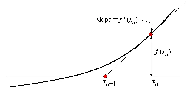
We draw a tangent line to the graph of f(x) at the point x=x_n ​. This line has slope f'(x_n) and goes through the point (x_n, f(x_n)). Therefore, it has the equation y = f'(x_n)*(x - x_n) + f(x_n). Now, we find the root of this tangent line by setting y = 0 and x=x_n+1​ for our new approximation. Solving this equation gives us our new approximation, which is `"x_(n+1)=x_n-(f(x)_(n))/(f'(x_n))"`

Ice sheet can be broken into small slabs with a heavy Air-Cushion Vehicle (ACV) travelling on the float ice sheet at a critical speed. Ice-breaking with ACV is a new ice-breaking method in the inland river that has an important application in the prevention of ice jam flood in the Yellow River. Dependent on ice thickness, an ACV can readily break the ice in flexure by making depression and send cracks through the ice. Once a crack is made, the path of least resistance for the ACV's air curtain gets under the ice and reduces the supporting water under the ice. The ice then falls under its own weight. At speed, an ACV can setup a wave in the ice and send cracks through it. This would act similar to the dynamics of a transport truck on an ice road.

GOVERNING EQUATIONS:

Where,

p denotes the cushion pressure,

h the thickness of the ice field,

r the size of the air cushion,

σ the tensile strength of the ice &

β is related to the width of the ice wedge.

INPUTS:

β = 0.5,

r = 40 feet &

σ = 150 pounds per square inch (psi).

STEPS (WITH EXPLANATION):

First, we import important modules viz are math, NumPy (as np), mathplotlib.pyplot (as plt) and provide initial inputs viz. width of the ice-wedge (beta), size of the air cushion (r), tensile strength of the ice in psi (alpha). We convert the tensile strength of the ice from pound per square inches (psi) to pound per square feet (PSF). The conversion is 1 foot = 12 inches; Therefore, 1 square feet = 12*12 square inches. The final result is alpha = 21600 pound per square feet. We also provide with an array of the thickness of the ice field (h) and an assumed value of the relaxation factor of 0.7.

Then we define two functions namely f and f_1 according to the formula and three empty arrays are created for storing values of pressure (in psi and psf) and a number of iterations.

Now we apply a for loop for calculating minimum pressure for different values of ice thickness taking an initial guessed value of pressure, tolerance and a loop counter =1 which will increment after every iteration is set. Then a while loop is initiated inside the same loop for checking whether all inputs in the formula if is greater than the tolerance provided, a new value of pressure will be calculated according to the Newton Raphson method. Then the values of pressure for psi and psf, and the number of iterations are stored in an array by using the append command. Some values are printed out which are the thickness of ice-wedge, cushion pressure (in psi and psf) and the number of iterations.

Then we plot two plots for pressure vs thickness of ice field. In the first plot pressure is taken in PSF and in the second plot pressure is taken in psi. Plot title, labels and grid are provided in the plot.

For calculating the optimal relaxation factor for a given value of the thickness of ice, the same steps as above are repeated except now an array of alpha ranging from 0.1 to 1.9 is taken with 50 points in between them and h = 0.6 is taken. Same for loop and while loop is again executed for checking whether all inputs in the formula are greater than tolerance provided; A new value of pressure will be calculated according to the Newton Raphson method. The number of iterations calculated is stored as an array and a graph is plotted between the same and relaxation factors. Plot title, labels and grid are provided.

CODE:

'''
A program to calculate pressure for given thickness of ice using Newton Raphson Method
By Utkarsh Palwekar
'''

import math
import numpy as np
import matplotlib.pyplot as plt

# Inputs
beta = 0.5 # beta  is related to the width of the ice wedge
r = 40 # r is the size of the air cushion (feet)
alpha = 150 # alpha the tensile strength of the ice (pounds per square inch (psi))
''' alpha the tensile strength of the ice (pounds per square foot)
    1 foot = 12 inches
    1 square feet = 12*12 square inches'''
alpha = 21600
h = [0.6, 1.2, 1.8, 2.4, 3.0, 3.6, 4.2] # h the thickness of the ice field
r_f = 0.7 # Relaxation factor assumed


def f(p, h, r, beta, alpha):
    term_1 = pow(p, 3) * (1 - pow(beta, 2))
    term_2a = 0.4 * h * pow(beta, 2)
    term_2b = (alpha * (pow(h, 2)) / pow(r, 2))
    term_3 = pow(alpha, 2) * (pow(h, 4)) / (pow(r, 4))
    term_4 = (alpha / 3) * (pow(h, 2)) / (pow(r, 2))

    return term_1 + (term_2a - term_2b) * pow(p, 2) + term_3 * (p / 3) - pow(term_4, 3)


def f_1(p, h, r, beta, alpha):
    term_5 = 3 * pow(p, 2) * (1 - pow(beta, 2))
    term_6a = 0.4 * h * pow(beta, 2)
    term_6b = (alpha * (pow(h, 2)) / pow(r, 2))
    term_7 = pow(alpha, 2) * (pow(h, 4)) / (pow(r, 4))

    return term_5 + 2 * (term_6a - term_6b) * p + term_7 / 3


# Null pressure array for storing calculated values after each iterations
pressure_psf = []  # pound per square feet
pressure_psi = []  # pound per square inches(psi)

# Null array for storing the number of iterations in future
num = []

for i in h:

    # Assuming initial pressure value
    p_guess = 100

    # Tolerance
    tolerance = 1e-5

    # Loop counter for incrementing the number of iterations
    counter = 1

    while (abs(f(p_guess, i, r, beta, alpha)) > tolerance):
        p_guess = p_guess - r_f * (f(p_guess, i, r, beta, alpha) / f_1(p_guess, i, r, beta, alpha))
        counter = counter + 1

    pressure_psf.append(p_guess)
    pressure_psi.append(p_guess / 144)
    num.append(counter)

print('Thickness of the Ice wedge :', h)
print('Cushion Pressure (pound per square feet) :', pressure_psf)
print('Cushion Pressure (psi) :', pressure_psi)
print('Number of iterations :', num)

# Plotting graph
plt.figure(1)
plt.plot(h, pressure_psf, marker='o', color='black', markerfacecolor='blue')
plt.title('Cushion Pressure vs Ice Field Thickness')
plt.xlabel('Thickness of Ice Field (feet)')
plt.ylabel('Cushion Pressure (pound per square feet)')
plt.grid()
plt.show()

plt.figure(2)
plt.plot(h, pressure_psi, marker='o', color='black', markerfacecolor='green')
plt.title('Cushion Pressure vs Ice Field Thickness')
plt.xlabel('Thickness of Ice Field (feet)')
plt.ylabel('Cushion Pressure (pound per square inches)')
plt.grid()
plt.show()

''' The program to calculate optimal relaxation factor for given thickness of ice field'''

# h_1 the thickness of the ice field
h_1 = 0.6
# Relaxation factor array assumed considering underrelaxing and overrelaxing values
r_f_array = np.linspace(0.1, 1.9, 50)
# Null array for storing the number of iterations in future
num_1 = []

for j in r_f_array:

    # Assuming initial pressure value
    p_guess = 100

    # Tolerance
    tolerance = 1e-5

    # Loop counter for incrementing the number of iterations
    counter = 1

    while (abs(f(p_guess, h_1, r, beta, alpha)) > tolerance):
        p_guess = p_guess - (j * f(p_guess, h_1, r, beta, alpha)) / f_1(p_guess, h_1, r, beta, alpha)

        counter = counter + 1

    num_1.append(counter)
    print(j)

# Plotting graph
plt.figure(3)
plt.plot(r_f_array, num_1, marker='.', color='black', markerfacecolor='red')
plt.xlabel('Relaxation Factor')
plt.ylabel('No. of Iterations')
plt.title('Iterations vs Relaxation Factor')
plt.grid()
plt.show()

 

RESULTS/OUTPUT:

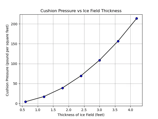
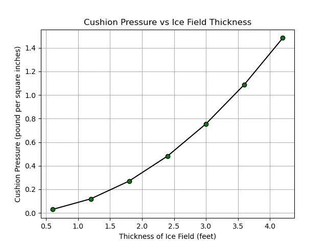
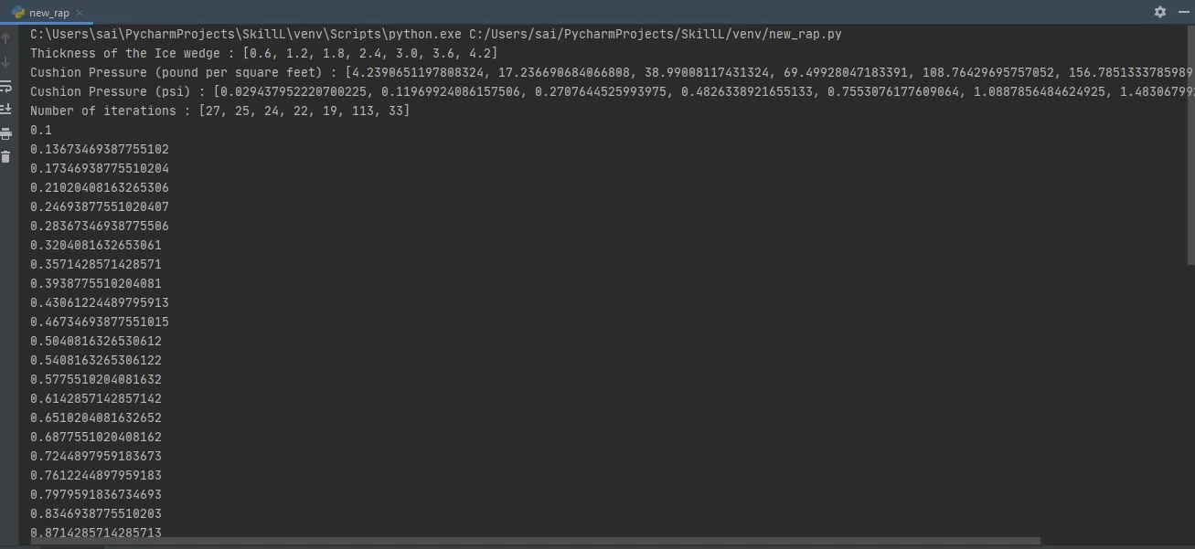
The program yields pressure values for different ice thicknesses. From here it was observed that when ice thickness was 0.6, the pressure corresponding to it was 4.24 psf or 0.0294 psi.

Cushion Pressure (pound per square feet) vs Ice Field Thickness Plot. It shows the variation of pressure with ice thickness.

Cushion Pressure (pound per square inches) vs Ice Field Thickness Plot

Iteration vs Relaxation Factor plot

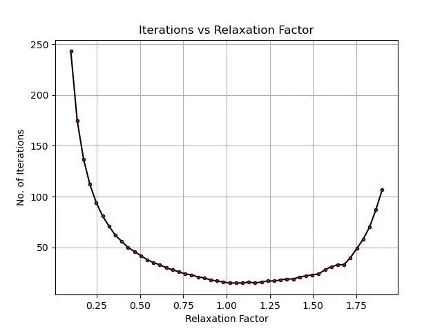
From the above plot, we can find the optimal value of factor relaxation for the given ice field thickness. Here we can observe that as the number of iterations increases the relaxation factor increases and began to converge near 1 and again increases with the number of iterations. Hence, we can derive that the value of the relaxation factor lies nearby the value of 1. It could be somewhere between these values -

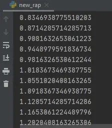
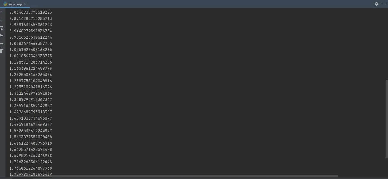
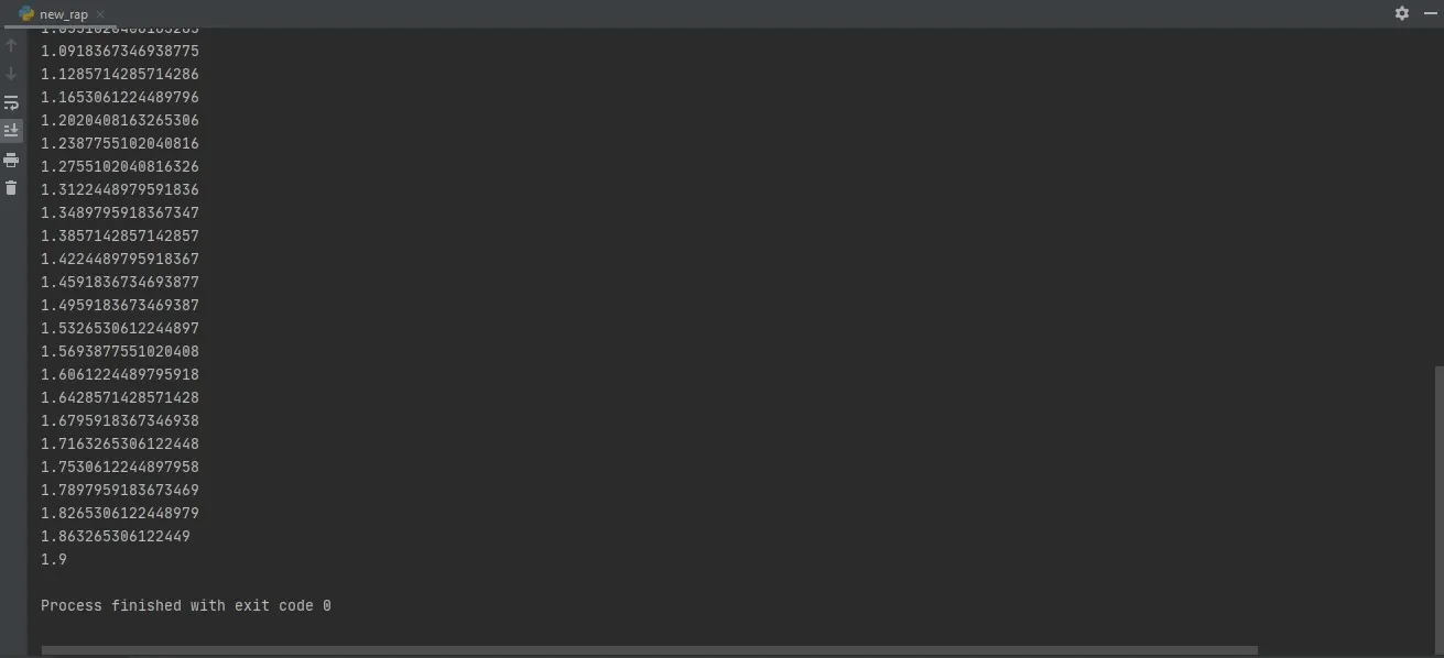
Output in run window-

CONCLUSION:

By running this program or code we can conclude that the Newton Raphson method is a powerful method for calculating solutions for non-linear functions as it is a faster technique and gives approximately close solutions in fewer iterations compared to other methods.

ERRORS & SOLUTION:

Few typo errors and indentation errors were encountered which was solved by revaluation the code.

REFERENCES:

https://en.wikipedia.org/wiki/Newton%27s_method

https://brilliant.org/wiki/newton-raphson-method/

https://globalnews.ca/news/6630036/coast-guard-hovercraft-breaks-ice-chateauguay-river/