Project - Speed Control of a Direct Current (DC) motor
Q. No.- 01: DC Motor with Controller Design
What is a DC Motor?
A DC motor defined as a class of electrical motors that convert electrical direct current electrical energy into mechanical energy.
From the above definition, we can conclude that any electric motor that is operated using direct current or DC is called a DC motor. We will understand the DC motor construction and how a DC motor converts the supplied DC electrical energy into mechanical energy in the next few sections.
DC Motor Diagram
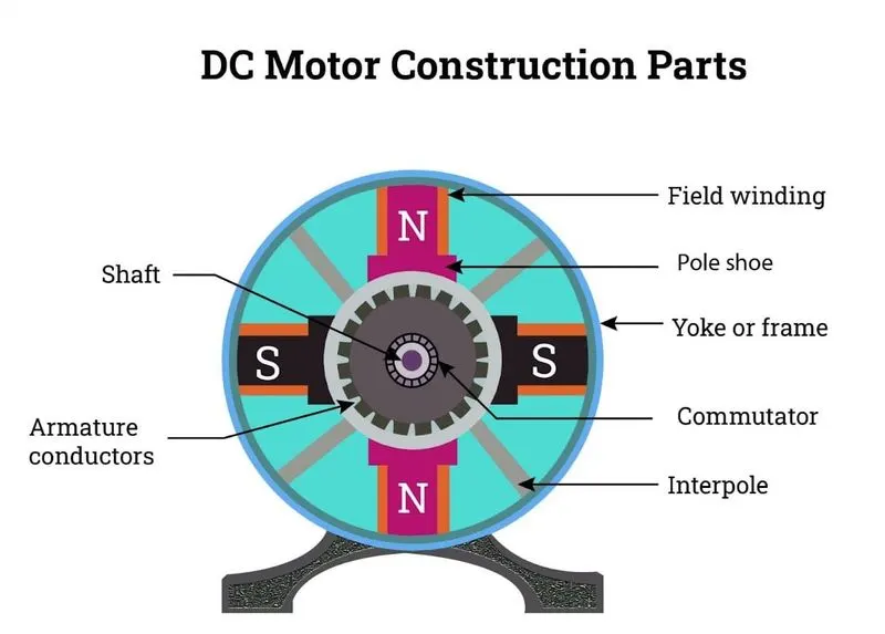
Different Parts of a DC Motor:
A DC motor is composed of the following main parts;
1.Armature or Rotor:
The armature of a DC motor is a cylinder of magnetic laminations that are insulated from one another. The armature is perpendicular to the axis of the cylinder. The armature is a rotating part that rotates on its axis and is separated from the field coil by an air gap.
2.Field Coil or Stator:
A DC motor field coil is a non-moving part on which winding is wound to produce a magnetic field. This electro- magnet has a cylindrical cavity between its poles.
3.Commutator:
The commutator of a DC motor is a cylindrical structure that is made of copper segments stacked together but insulated from each other using mica. The primary function of a commutator is to supply electrical current to the armature winding.
4.Brushes:
The brushes of a DC motor are made with graphite and carbon structure. These brushes conduct electrical current from the external circuit to the rotating commutator. Hence, we come to understand that the commutator and the brush unit are concerned with transmitting the power from the static electrical circuit to the mechanically rotating region or the rotor.
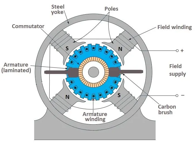
DC Motor Working:
A magnetic field arises in the air gap when the field coil of the DC motor is energised. The created magnetic field is in the direction of the radii of the armature. The magnetic field enters the armature from the North pole side of the field coil and exits the armature from the field coils South pole side.
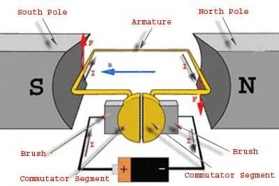
The conductors located on the other pole are subjected to a force of the same intensity but in the opposite direction. These two opposing forces creat a torque that causes the motor armature to rotate.
Principle:
When kept in a magnetic field, a current carrying conductor gains torque and develops a tendency to move. In short, when electric fields and magnetic fields interact, a mechanical force arises. This is the principle on which the DC motors work.
What is a PID Controller?
A PID controller is an instrument used in industrial contorl applications to regulate temperature, flow, pressure, speed and other process variables. PID controllers use a control loop feed back mechanism to control process variables and are the most accurate and stable controller.
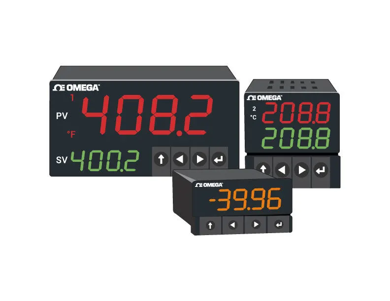
PID control is well-established way of driving system towards a target position or level. It's practically ubiquitous as a means of controlling temperature and finds application in myriad chemical and scientific process as well as automation. PID control uses closed -loop control feedback to keep the actual output from a process as close to the target or setpoint output as possible.
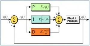
PID Controller Block Diagram:
A closed-loop system like a PID controller includes a feedback control system. This system evaluvates the feedback variable using a fixed point to genrate an error signal. Based on that, it alterrs the system output. This procedure will continue till the error reaches zero otherwise the value of the feedback variable becomes equivalent to a fixed point.
Working of PID Controller:
The basic idea behind a PID controller is to read a sensor, then compute the desired actutator output by calculating proportional, integral and derivative responses and summing those three components to compute the output.
P- Controller:
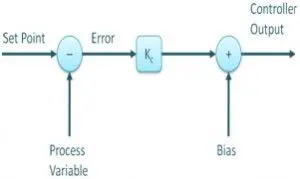
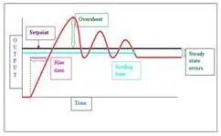
Proportional or P- controller gives an output that is proportional to current error e(t). It compares the desired or set point with the value or feedback process value. The resulting value multiplied with a proportional constant to get the output. If the error value is zero, then this controller output is zero.
P-Controller P-Controller Response
This controller requires biasing or manual reset when used alone. This is because it never reaches steady -state condition. It provides stable operation but always maintains the steady-state error. The speed of the response is increased when the proportional consatnt Kc increases.
I-Controller:
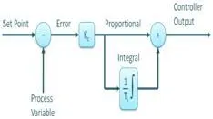
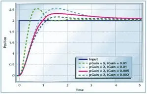
Due to the limitation of P-controller where there always exists an offset between the process variable and setpoint, I-controller is needed, which provides necessary action to eliminate the steady state error. It integrates the error over period of time until the error value reaches zero. It holds the value to the final control device at which error becomes zero.
PI-Controller PI-Controller Response
Integral control decreases it's output when a negative error takes place. It limits the speed of response and affects the stability of the system. The speed of the response is increased by decreasing integral gain,Ki.
D-Controller:
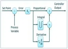
I-controller doesn't have the capability to predict the future behavior of error. So it reacts normally once the setpoint is changed. D-controller overcomes this problem by anticipating the future behavior of the error. Its output depends on the rate of change of error with respect to time, multiplied by derivative constant. It gives the kick start for the output there by increasing system response.
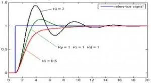
PID-Controller PID-Controller Response
So finally we observed that by combining these three controllers, we can get the desired response for the system. Different manufactures design different PID algorithms.
Mathematical Model of DC Motor
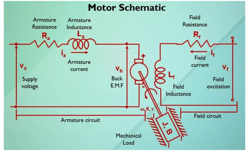
For this above schematic Diagram ,we will assume the Input odf the dc moter is Voltage source(Vs) and out of the moter is Rotational speed (w) of the moter shaft.
Both the rotor and shaft are to rigid then we gets the Viscus friction(J) and Tarque(T).
The Tarque (T) of the motor is prapotional to the armature Current (ia) with tarque Constant (Kt)
i.e., T=Kt * ia-----------(1)
Back EMF (Vb) is praportional to angular velocity (theta_dot) by a praportional constatnt (Kb)
i,e., Vb = Kb * (theta_dot)----------(2)
For creating the The SIMULINK MODEL of above given DC moter let us find the transfer funcion as followes ::-
From the schematic diagram we have apply kirchoff's Voltage law To the Armature Circuit as Given below:-
Armature Circuit Equatation Part :-
Vs= Ra* ia + L (dia/ dt) +Vb ----------(3)
substitute eqn (2) in eqn (3) then we get
Vs= Ra* ia + L (dia/ dt) +(Kb* (theta_dot)-----------(4)
Vs-(Kb* (theta_dot)=Ra* ia + L (dia/ dt)------------(5)
From Equatation (5) we can write as :-
L( d ia / dt ) = (Vs-(Kb* (theta_dot)-Ra*ia)-----------(6)
Field Circuit Equatation Part:-
Appling the Newton's Law of Moton for Field circuit Then we get:-
J(d^2 theta /d t^2) + B (d theta /d t)= Kt * ia---------------(7)
Apply Laplace Transforms to both equatations (6) and (7) then :-
from eqn (6) :-
L I(S)=V(S)- Kb (theta (S)- Ra I(S)
L I(S)+ Ra I(S)=V(S)- Kb (theta (S))
I(S) (L+Ra)=V(S)- Kb (theta (S))
I(S)=V(S)- Kb (theta (S) / (L+Ra)-----------------(8)
From eqn (7):-
J S^2 (theta (S))+ B s (theta (S)) =kt * I(S)---------------(9)
substitute I(S) value in eqn (9) then we get :-
J S^2 (theta (S))+ B s (theta (S)) =kt *{V(S)- Kb (theta (S) / (L+Ra)}
S * theta (S) ( J S +B)=kt *{V(S)- Kb (theta (S) / (L S+Ra)}---------------------(10)
From equatation (10):-
We get transfer function between output (w(s)) Angular velocity and input volatge (Vs) as followes :-
W(S) / Vs = Kt / {(L S+Ra) (J S + B)+Kt* Kb}-----------------(11)
Mathematical modeling from the first principles:-
From eqn (11):-
This we can design the SIMULINK MODEL:-
W(S) / Vs = Kt / {(L S+Ra) (J S + B)+Kt* Kb}
Block Used:
Step - The Step block provides a step between two definable levels at a specified time. If the simulation time is less than the Step time parameter value, the block's output is the Initial value parameter value.
Sum - The Sum block performs addition or subtraction on its inputs. This block can add or subtract scalar, vector, or matrix inputs. It can also collapse the elements of a single input vector.
Gain - The Gain block multiplies the input by a constant value (gain). The input and the gain can each be a scalar, vector, or matrix.
Integrator - The Integrator block outputs the integral of its input at the current time step.
Derivative - Output the time derivative of the input. It approximates the derivative of its input by computing.
Transfer Function - It implements a transfer function where the input (u) and output (y) can be expressed in transfer function form
Clock - Outputs the current simulation time at each simulation step and useful for other blocks that need the simulation time.
to Workspace - Write data to the workspace. Writes its output to an array or structure that has the name specified by the block's Variable name parameter.
Logic:
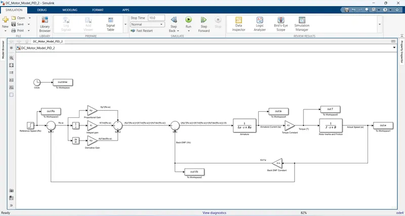
For 1st term (Rs-w), w subtracted from Rs using Sum block
For 2nd term Kp*(Rs-w), (Rs-w) is multiplied with Kp using Gain block
For 3rd term Ki*int(Rs-w), (Rs-w) is passed through Integrator block then multiplied with Ki using Gain block
For 4th term Kd*der(Rs-w), (Rs-w) is passed through Derivative block then multiplied with Kd using Gain block
For 5th term (Kp*(Rs-w))+(Ki*int(Rs-w))+(Kd*der(Rs-w)), (Kp*(Rs-w)), (Ki*int(Rs-w)) and (Kd*der(Rs-w)) is added using Sum block
For 6th term (Km*w), w multiplied with Km using Gain block
For 7th term ((Kp*(Rs-w))+(Ki*int(Rs-w))+(Kd*der(Rs-w)))-(Km*w), (Km*w) is subtracted from ((Kp*(Rs-w))+(Ki*int(Rs-w))+(Kd*der(Rs-w))) using Sum block
Then it send through the Rotor Inertia and Friction or Transfer Function (1/La*s+Ra)
Then It multiplied with Kt using Gain block
Then it send through the Armature or Transfer Function (1/J*s+B)
Then it send back to 1st and 6th term.
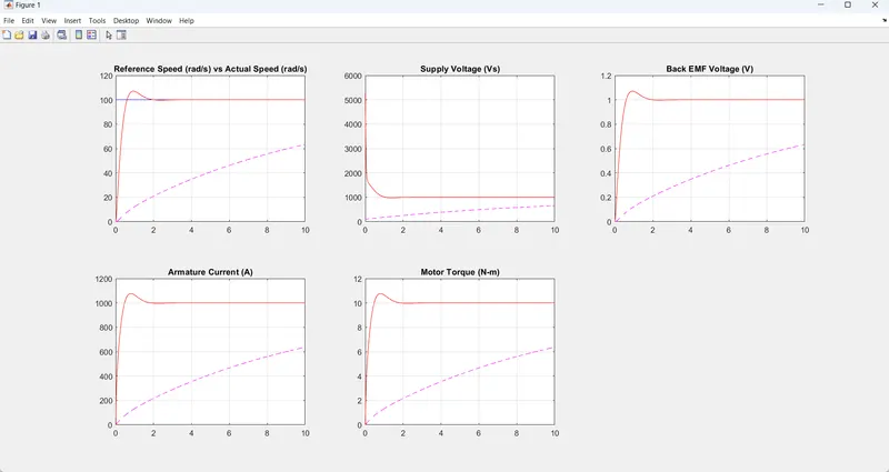
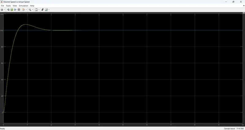
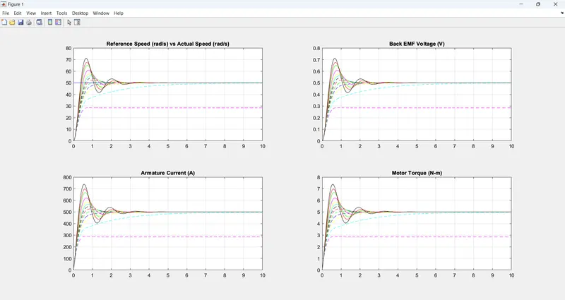
Here we take Reference Speed (Rs) as Step block in which Final Value = 50
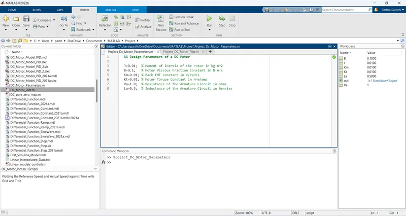
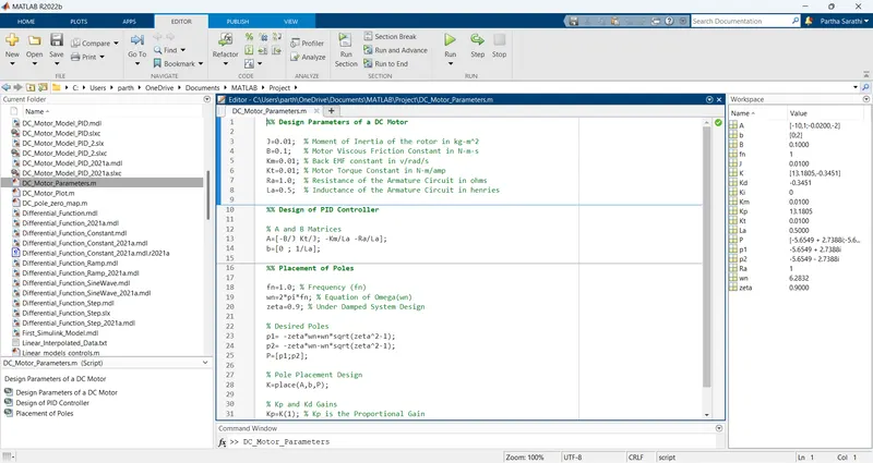
DC Motor Parameters Script:
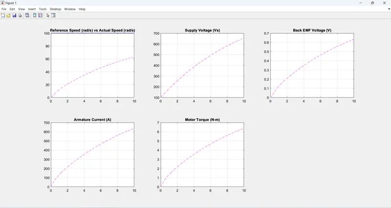
>> DC_Motor_Plot
>> Ki=10;
>> subplot(221); plot(out.time,out.w,'c--');
subplot(222); plot(out.time,out.Vb,'c--');
subplot(223); plot(out.time,out.Ia,'c--');
subplot(224); plot(out.time,out.T,'c--');
>> Ki=20;
>> subplot(221); plot(out.time,out.w,'y--');
subplot(222); plot(out.time,out.Vb,'y--');
subplot(223); plot(out.time,out.Ia,'y--');
subplot(224); plot(out.time,out.T,'y--');
>> Ki=25;
>> subplot(221); plot(out.time,out.w,'b--');
subplot(222); plot(out.time,out.Vb,'b--');
subplot(223); plot(out.time,out.Ia,'b--');
subplot(224); plot(out.time,out.T,'b--');
>> Ki=30;
>> subplot(221); plot(out.time,out.w,'g--');
subplot(222); plot(out.time,out.Vb,'g--');
subplot(223); plot(out.time,out.Ia,'g--');
subplot(224); plot(out.time,out.T,'g--');
>> Ki=35;
>> subplot(221); plot(out.time,out.w,'r--');
subplot(222); plot(out.time,out.Vb,'r--');
subplot(223); plot(out.time,out.Ia,'r--');
subplot(224); plot(out.time,out.T,'r--');
>> Ki=40;
>> subplot(221); plot(out.time,out.w,'k--');
subplot(222); plot(out.time,out.Vb,'k--');
subplot(223); plot(out.time,out.Ia,'k--');
subplot(224); plot(out.time,out.T,'k--');
>> Ki=45;
>> subplot(221); plot(out.time,out.w,'c-');
subplot(222); plot(out.time,out.Vb,'c-');
subplot(223); plot(out.time,out.Ia,'c-');
subplot(224); plot(out.time,out.T,'c-');
>> Ki=50;
>> subplot(221); plot(out.time,out.w,'y-');
subplot(222); plot(out.time,out.Vb,'y-');
subplot(223); plot(out.time,out.Ia,'y-');
subplot(224); plot(out.time,out.T,'y-');
>> Ki=60;
>> subplot(221); plot(out.time,out.w,'m-');
subplot(222); plot(out.time,out.Vb,'m-');
subplot(223); plot(out.time,out.Ia,'m-');
subplot(224); plot(out.time,out.T,'m-');
>> Ki=75;
>> subplot(221); plot(out.time,out.w,'g-');
subplot(222); plot(out.time,out.Vb,'g-');
subplot(223); plot(out.time,out.Ia,'g-');
subplot(224); plot(out.time,out.T,'g-');
>> Ki=85;
>> subplot(221); plot(out.time,out.w,'r-');
subplot(222); plot(out.time,out.Vb,'r-');
subplot(223); plot(out.time,out.Ia,'r-');
subplot(224); plot(out.time,out.T,'r-');
>> Ki=100;
>> subplot(221); plot(out.time,out.w,'k-');
subplot(222); plot(out.time,out.Vb,'k-');
subplot(223); plot(out.time,out.Ia,'k-');
subplot(224); plot(out.time,out.T,'k-');
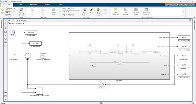
Block Used:
Step - The Step block provides a step between two definable levels at a specified time. If the simulation time is less than the Step time parameter value, the block's output is the Initial value parameter value.
Sum - The Sum block performs addition or subtraction on its inputs. This block can add or subtract scalar, vector, or matrix inputs. It can also collapse the elements of a single input vector.
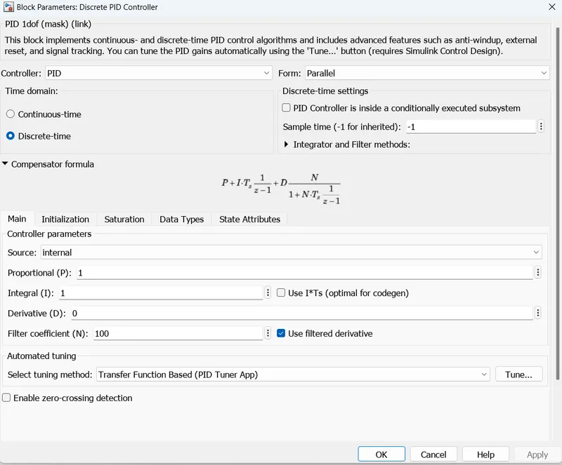
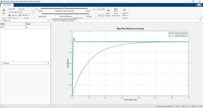
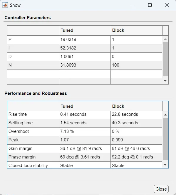
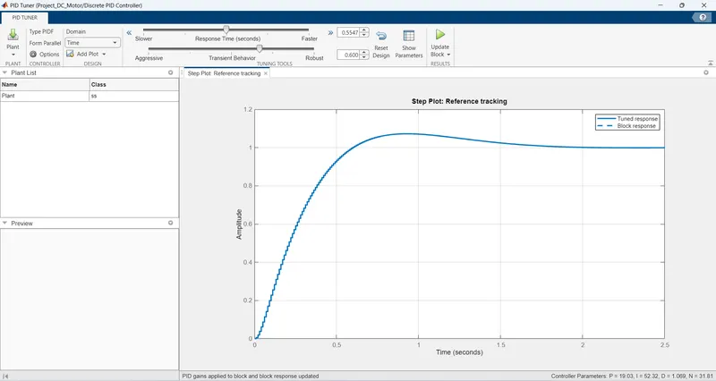
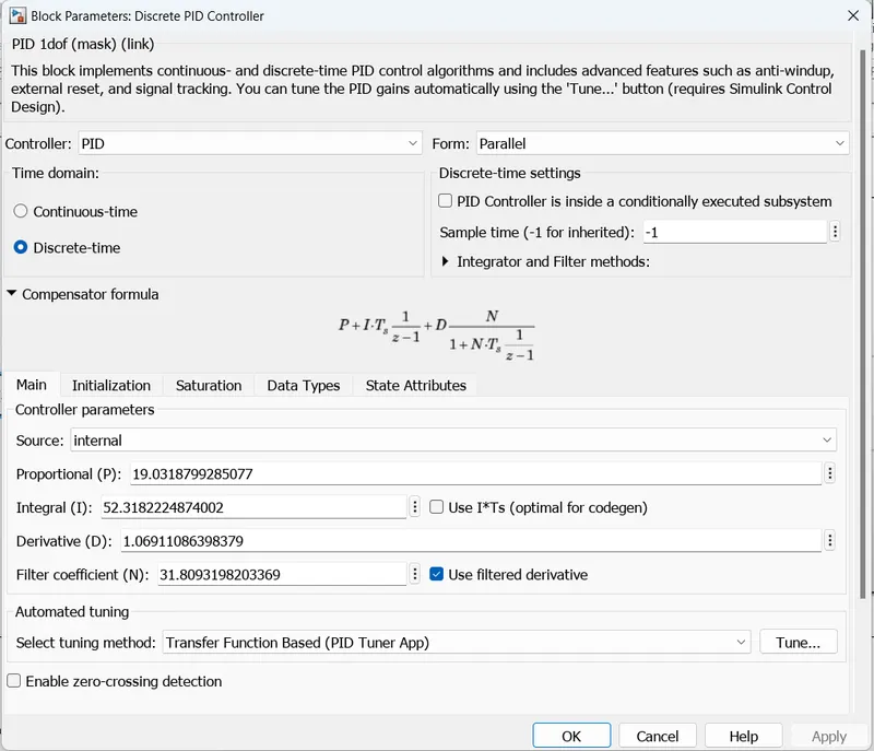
Discrete PID Controller - The PID Controller block implements a PID controller (PID, PI, PD, P only, or I only). The block is identical to the Discrete PID Controller block with the Time domain parameter set to continuous time.
The block output is a weighted sum of the input signal, the integral of the input signal, and the derivative of the input signal. The weights are the proportional, integral, and derivative gain parameters. A first-order pole filters the derivative action.
Gain - The Gain block multiplies the input by a constant value (gain). The input and the gain can each be a scalar, vector, or matrix.
Integrator - The Integrator block outputs the integral of its input at the current time step.
Derivative - Output the time derivative of the input. It approximates the derivative of its input by computing.
Transfer Function - It implements a transfer function where the input (u) and output (y) can be expressed in transfer function form
Zero Order Hold - The Zero-Order Hold block samples and holds its input for the specified sample period. The block accepts one input and generates one output, both of which can be scalar or vector. If the input is a vector, all elements of the vector are held for the same sample period.
Clock - Outputs the current simulation time at each simulation step and useful for other blocks that need the simulation time.
to Workspace - Write data to the workspace. Writes its output to an array or structure that has the name specified by the block's Variable name parameter.
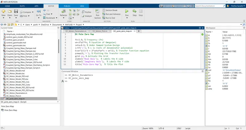
DC Motor Parameters Script: