Project - Speed Control of a Direct Current (DC) motor

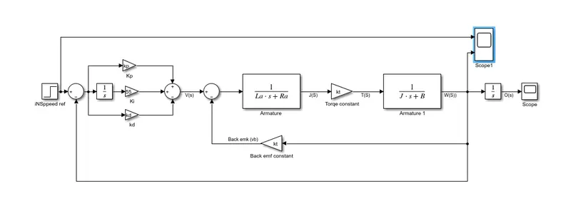
In this project, a Simulink model for the DC motor will be first developed per the schematic shown in Figure 1.

Use the Proportional, Integral, and Derivative (PID) control design knowledge gained in the training to design, develop and test a controller to maintain a desired speed for the motor.

Mathematical modeling from the first principles:

A common actuator in control systems is the DC motor. It directly provides rotary motion and, coupled with wheels or drums and cables, can provide translational motion.

For this example, we will assume that the input of the system is the voltage source () applied to the motor's armature, while the output is the rotational speed of the shaft . The rotor and shaft are assumed to be rigid. We further assume a viscous friction model, that is, the friction torque is proportional to shaft angular velocity.

The physical parameters for our example are:

(J)     moment of inertia of the rotor     0.01 kg.m^2

(b)     motor viscous friction constant    0.1 N.m.s

(Ke)    electromotive force constant       0.01 V/rad/sec

(Kt)    motor torque constant              0.01 N.m/Amp

(Ra)     Armature electric resistance                1 Ohm

(La)   Armature  electric inductance                0.5 H

Design requirements

First consider that our uncompensated motor rotates at 0.1 rad/sec in steady state for an input voltage of 1 Volt (this is demonstrated in the DC MOTOR where the system's open-loop response is simulated). Since the most basic requirement of a motor is that it should rotate at the desired speed, we will require that the steady-state error of the motor speed be less than 1%. Another performance requirement for our motor is that it must accelerate to its steady-state speed as soon as it turns on. In this case, we want it to have a settling time less than 2 seconds. Also, since a speed faster than the reference may damage the equipment, we want to have a step response with overshoot of less than 5%.

In summary, for a unit step command in motor speed, the control system's output should meet the following requirements.

State Space

We can also represent the system using the state-space equations. The following additional MATLAB commands create a state-space model of the motor and produce the output shown below when run in the MATLAB command window.

A = [-B/J   Kt/J
    -Km/La   -Ra/La];
B = [0
    1/La];


PID controller:

The output of a PID controller, which is equal to the control input to the plant, is calculated in the time domain from the feedback error as follows:

First, let's take a look at how the PID controller works in a closed-loop system using the schematic shown above. The variable () represents the tracking error, the difference between the desired output () and the actual output (). This error signal () is fed to the PID controller, and the controller computes both the derivative and the integral of this error signal with respect to time. The control signal () to the plant is equal to the proportional gain () times the magnitude of the error plus the integral gain () times the integral of the error plus the derivative gain () times the derivative of the error.

This control signal () is fed to the plant and the new output () is obtained. The new output () is then fed back and compared to the reference to find the new error signal (). The controller takes this new error signal and computes an update of the control input. This process continues while the controller is in effect.

Simulink based modeling

Matlab script to define modeling and control design parameters

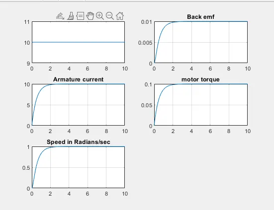
For the plot of design parameter:




Output of the model by pid controller on values of Kp,Ki and  Kd gains in the model

CL RESPONSE	RISE TIME	OVERSHOOT	SETTLING TIME	S-S ERROR
Kp	Decrease	Increase	Small Change	Decrease
Ki	Decrease	Increase	Increase	Decrease
Kd	Small Change	Decrease	Decrease	No Change

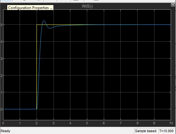
Increasing the proportional gain () has the effect of proportionally increasing the control signal for the same level of error. The fact that the controller will "push" harder for a given level of error tends to cause the closed-loop system to react more quickly, but also to overshoot more. Another effect of increasing is that it tends to reduce, but not eliminate, the steady-state error.

The addition of a derivative term to the controller () adds the ability of the controller to "anticipate" error. With simple proportional control, if is fixed, the only way that the control will increase is if the error increases. With derivative control, the control signal can become large if the error begins sloping upward, even while the magnitude of the error is still relatively small. This anticipation tends to add damping to the system, thereby decreasing overshoot. The addition of a derivative term, however, has no effect on the steady-state error.

The addition of an integral term to the controller () tends to help reduce steady-state error. If there is a persistent, steady error, the integrator builds and builds, thereby increasing the control signal and driving the error down. A drawback of the integral term, however, is that it can make the system more sluggish (and oscillatory) since when the error signal changes sign, it may take a while for the integrator to "unwind."