Project - Speed Control of a Direct Current (DC) motor

Electrical Engineering System

Motor

Electrical Energy is convert to Mechanical Energy it use of torque generated for loads move on and lift on purpose also it most mechanical purpose to used.

They are Three types of motor,

Also Motor is run Flemming Left Hand Rule

Whenever a current carrying conductor is placed in a magnetic field, it experiences a mechanical force.

F= BIL Newton

B = magenetic flux density; I= current; L= length of the conductor within the magentic field

1.Dc Motor 2.Ac Motor 3.Special Motor

Dc Motor (Direct Current) that also Two Types

1. Brushless Dc Motor(Core less or Iron loss Dc Motor)

2.Brush Dc Motor(1.Separately Excited; 2.Self Excited; 3. Permanent Magnet; 4. Servo Motor 5.Universal Motor

Self Excited Dc Motor also three Main Types(1.Shunt Wound; 2.Series Wound; 3.Compound Wound(short wound and long wound)

Here, topic of Dc Motor Speed Control also they are Two Types;

1.Field Current Control Method (If) or Constant Power Region

Field Current Control Method is Vary of Field current to be control of Speed on Motor, Speed to be control of above rated speed of motor Speed

2.Armature Current Control Method (Ia) or Constant Torque Region

Armature Current Control Method is Vary of Armature current to be control of Speed on Motor, Speed to be control of below rated speed of motor Speed

Dc motor Back E.m.f

Eb = P*pi*Z*N/60A

P- Number of Poles - Constant

pi-Flux(Field Control) - Variable

Z-Number of Conductor - constant

N- RPM - Variable

A-Types of Winding(lap Winding A=P or Wave Winding A=Z) - constant

separate of Constant,

Eb= (pz/60A)*pi N

Eb = k * pi* N (k- constant)

pi = Eb/N or (pi&1/N) Speed and Flex is inversly Propotional

Speed Increase Flex Decrease; Flex Increase Speed Decrease

Vt = Eb + IaRa

Eb = Vt - IaRa

Here,Ia will Change Eb Change

Eb depends upon Speed(w or N), current (Ia) ,flex(pi)

Torque propotional(&) pi*Ia

Dc motor speed control oriented on torque and Eb

1.Field current(If) will decrease and flex decrease(pi) Speed(N) Increase

Field Current Depends on Field flex so this Above rated speed control

This method called Field weekining method

2.Armature Current (Ia) will be Increase and Back Emf(Eb) Decrease Speed(N) Decrease so this below rated speed control

Here We will Discuss (Simulink and MATLAB) DC Servo Motor

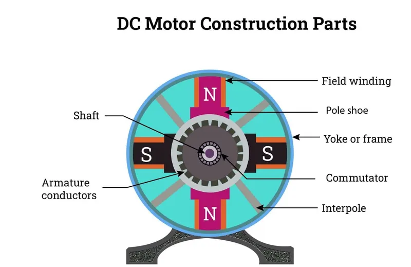
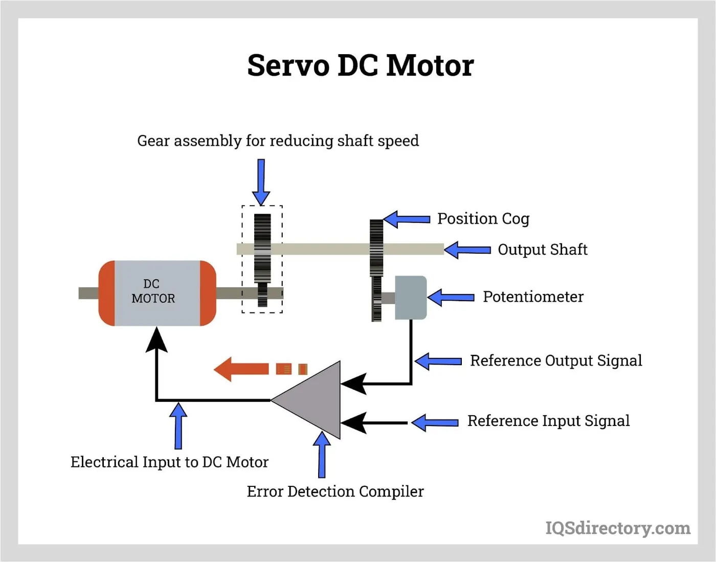
A servo DC motor has four parts: a DC motor, gearbox, control circuit, and position sensing unit. The gearbox changes high speed input into slower practical speed. The control circuit is an error detector amplifier. The position of the shaft gives feedback to the control circuit and is in a closed loop. With a servo DC motor, if there is any mismatch between the current position of the shaft and its reference position, an error signal is sent to the error detecting amplifier.

Servo Motor Use of minium voltage to be running also we will here Simulink and MATLAB step command (ex- 10V,20V,30V,40V and 230V)

there two circuit 1.Armature Circuit 2.Field circuit

Given supply from Armature Circuit then apply instantly 230v supply may coil failure,because at the time Armature Resistance and Armature Inductance so step step apply voltage or starter motor use the starting pupose.

Using kvl,

Vs = Ra ia + La dia/dt +Vb

Km = Kt= torque constant

w(s)/v(s)= Kt/(Js+B)*(Ls+B)+(KtKb)

Proportional ,Integral, Derivative

We know Pole Placement design of Matlab Fuction is called PLACE to determine the closed loop poles of spring mass system. Now, us find specific design objectivies of PID.control design individual gains.

PID control gains function of the regulation or Tracking Performance.

they are four type,

1.Rise Time 2. Setting Time 3. Overshoot 4.Steady state Error

Trasnfer Function of Angular Velocity w(s) to the V(s)

w(s)/v(s)= Kt/(Js+B)*(Ls+B)+(KtKb)