Project - Position control of mass spring damper system

Obtain the transfer function of a mass spring damper system and use it in the model. Add a PID controller to adjust the force on mass so that its position follows a reference signal.

Take m = 3.6 kg k = 400 N/m c = 100 Ns/m

Sol:

Transfer function of the Mass Spring Damper system:

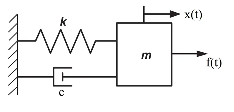
The above diagram is the graphical representation of spring mass damper system.

Here m = mass

k = spring constant

c = damping co efficient

f(t) = External force applied on the system

x(t) = Displacement of the system

By appling the Newton's 2nd law on the above system we can get

f(t) - c`dx/dt` - k x(t) = m `(d^2 x)/ dt^2` ----------> eq.1

By applying laplace transform on above equation

F(s) - csX(s) - kX(s) = m`s^2`X(s)

`nbsp; F(s) = (m`s^2`+ cs + k) X(s)

From above equation we get the transfer function X(s)/F(s) = 1/(ms^2 + cs + k) ------> eq.2

State Space model of the Spring Mass Damper System:

State variables X1(t) = x(t)

X2(t) = x.(t)

Input u(t) = f(t)

Output y(t) = x(t)

The eq.1 can be re write as below

u(t) - cX2(t) - kX1(t) = m x2.(t)

X1.(t) = X2(t)

`X2.(t) = -k/m X1(t) - c/m X2(t) + 1/m u(t)`

y(t) = X1(t)

From the above eq's we get the jacobian matrixes

A `=[[0,1], [-k/m,-c/m]]`

B `= [[0],[1/m]]`

Finding the Zeta & Natural Frequency:

By comparing the eq.2 with general transfer function, we get

wn^2 = k/m;

wn = sqrt(k/m);

`2 zeta wn` = c/m;

`zeta` = `c / (2m*wn)`

The matlab code for zeta Natural frequency, Propotional gain (Kp), Derivative gain (Kd) and Integral gain(Ki) calculations as shown below

clear;
clc;
% Parameters of the spring mass damper system
m = 3.6;
k = 400;
c = 100;
% finding the natural frequency and zeeta values
wn = sqrt(k/m);
zeta = c/(2*m*wn);
% the jacobian matrices
A = [0 1; -k/m -c/m];
B = [0;1/m];
% Pole placement method to find the prapotional & derivative gains (Kp & Kd)
a = 2*zeta*wn;
b = wn^2;
P = roots([1 a b]);
K = place(A,B,P);
Kp = K(1);
Kd = K(2);
% integral gain(Ki)
Ki = 750;

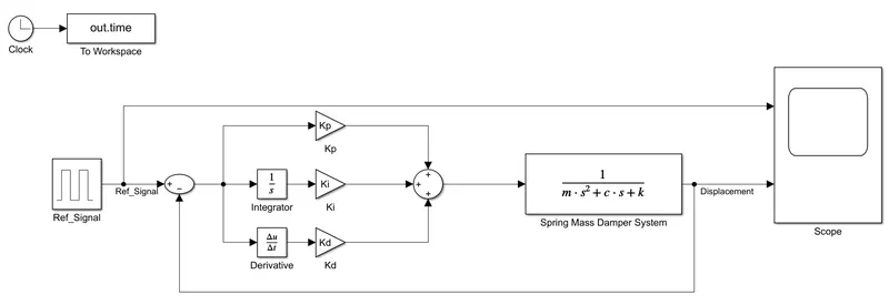
The simulink model is as shown below

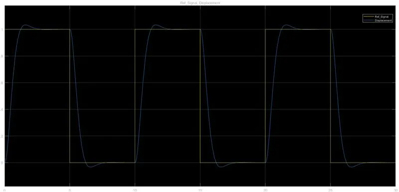
The generated displacement and the refference signal is as show below

Please find attached files for the matlab file, simulink model and the generated output.