Project - Position control of mass spring damper system
Aim:To design the transfer function of mass spring damper system and add a pid controller.
Objectives:
transfer function of a mass spring damper system and use it in the model. Add a PID controller to adjust the force on mass so that its position follows a reference signal. the matlab model of the pid control and transfer function pulse wavefrome generator.
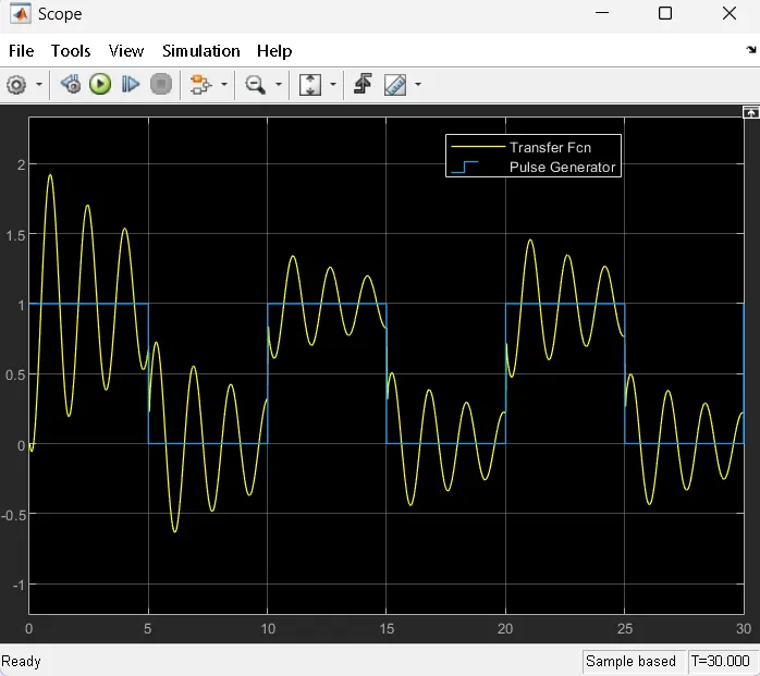
This example shows a controlled mass-spring-damper. A controller adjusts the force on the mass to have its position track a command signal. The initial velocity for the mass is 10 meters per second. The controller adjusts the force applied by the Force Source to track the step changes to the input signal.
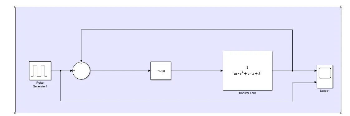
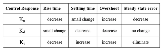
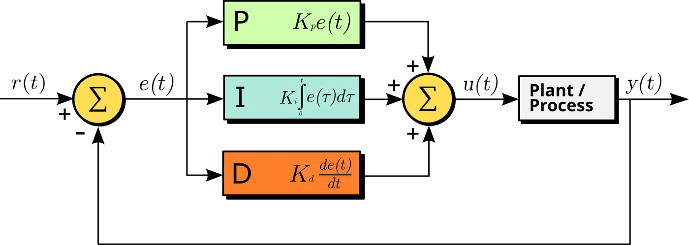
PID controller
In this project, PID controller has been designed by using Simulink in order to control a mass spring damper system which can move any direction. A transfer function for dc motor was added on the diagram. Response curve of the PID controller were fixed by tuning. The computer interface, different control algorithms can be performed on the system easily; control parameters can be set up online, filter algorithms in various structures can be tried and the reaction of these changeable values to the system can be observed. The effects of controller Proportional Integral Derivative (PID) for developing
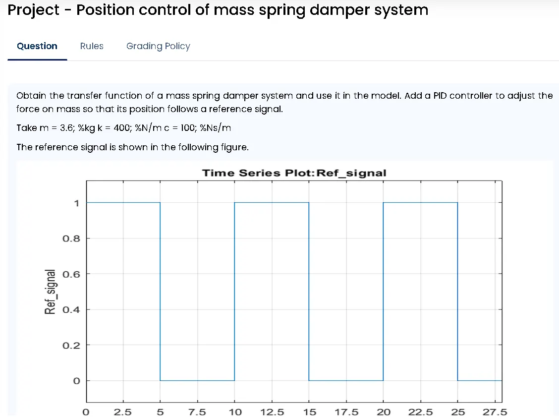
Obtain the transfer function of a mass spring damper system and use it in the model. Add a PID controller to adjust the force on mass so that its position follows a reference signal.
Take m = 3.6; %kg k = 400; %N/m c = 100; %Ns/m
Procedure:
The mass-spring-damper model consists of discrete mass nodes distributed throughout an object and interconnected via a network of springs and dampers. This model is well-suited for modelling object with complex material properties such as nonlinearity and viscoelasticity. Packages such as MATLAB may be used to run simulations of such models.As well as engineering simulation, these systems have applications in computer graphics and computer animation.
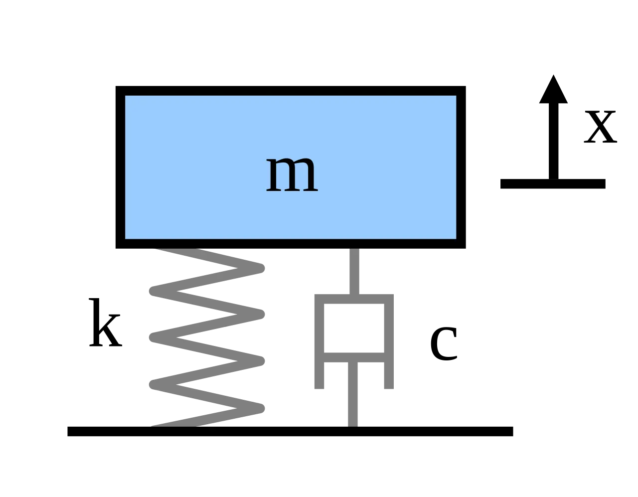
Force Equation for Spring Damper Mass System is
>> f(x) = m*x_dotdot + c*x_dot +k*x --------> (1)
where ' m ' is the mass of the Body
' k ' is the Spring stiffness constant
' c ' is the Damping Constant.
Apply Laplace transform on both sides of equation (1)
therefore
>> F(S) = m*s⊃2; *X(s) + c*s*X(S) + k*X(S)
where F(S) is the transfer function of the f(x)
X(S) is the transfer function of the x(t)
>> F(S) = X(S) [ m*s⊃2; + c*s + k ]
>> X(S)/F(S) = 1/ [ m*s⊃2; + c*s + k ] ----->(2)
equation (2) is the transfer function of the spring mass damper system.
Given Data:
- mass " m " = 3.6 kg
- Spring constant " k " = 400 N/m
- Damping constant " c " = 100 Ns/m
We know state matrix and Input matrix for the spring mass damper system are
- A = [ 0 1; -k/m -c/m ]; A is the state matrix
- A = [ 0 1; -111.111 -27.7778];
- B = [ 0 ; 1/m ] ; B is the Input matrix
- B = [ 0 ; 0.2778 ] ;
- let say zeta = 0.5 (under damped condition )
- angula frquency "wn" = sqrt (k/m) = 10.5409;
To finout the poles the following formula is used
- P1 = -zeta * wn + wn *sqrt (zeta⊃2;-1);
- P2 = -zeta * wn - wn *sqrt (zeta⊃2;-1);
- P = [ P1 ; P2 ];
Now we need to findout the Gains of the system like propotional gain and derivative gains using the place command.
therefore >> K = place(A,B,P)
where " A " is the state matrix of the Spring Mass Damper System.
" B " is the Input matrix of the Spring Mass Damper System.
" P " is the poles of the system
" K(1) " is the propotional Gain
" K(2) " is the derivative Gain
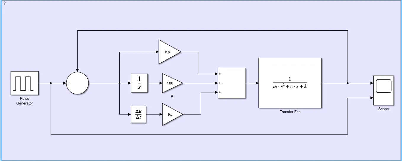
Building the Simulink model for positon control of Spring Mass Damper System with the Help of the Given Data
Block required for the Model are:
1. Pulse Generator Block : Used To give reference signal to the mass Spring Damper System.
2. Sum Block : Used To add the Simulink Signals
3. Gain Block: Gain Block is used to muliply the signal with a constant gain value.
4. Integrator Block: Integrator Block is Used to Integrate Input signal to it to get the required output of the signal.
5. Derivative Block: Derivative Block is used to Differentiate the input signal with respect to time.
6. Scope Block: Scope Block is Used to plot the required signal with respect to time.
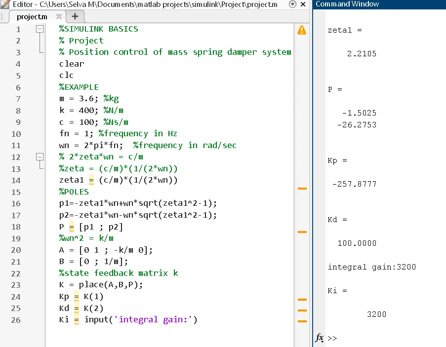
7. Transfer function Block: The transfer function block models a linear system by a transfer function of the Laplace-domain variable S. The Block can model single-input single-output(SISO) and single-input multiple-output(SIMO) systems.
Modeling a Single-Output System
For a single-output system, the input and output of the block are scalar time-domain signals. To model this system:
1. Enter a vector for the numerator coefficients of the transfer function in the Numerator coefficients field.
2. Enter a vector for the denominator coefficients of the transfer function in the Denominator coefficients field.
Trasnfer function:
The first thing is setting up the transfer function.Set the initial velocity as 10m/s.The controller adjust the force applied by itself. Trasnfer function of a mass spring damper system and use it in the model. Add a PID controller to adjust the force on mass so that its position follows a reference signal. The matlab model of the pid control and transfer function pulse wavefrome generator.
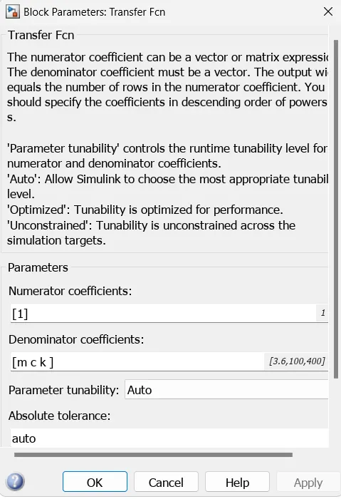
Writing the MATLAB CODE for the Model Positioon Control Spring Mass Damper System is shown below.
Simulink Model for the Position control of Spring Mass Damper System with manual PID Controller
Explanation:
- Here we subtracting the reference Signal from the Feedback Signal and the resulting signal is represented as the error Signal.
- Error Signal is Passes through the PID Controller with Proportional Integral and Derivative gains.
- In the Function Block set the Denominator Coefficients mass " m ", Damping Coefficient " c ", and Spring Constant " k ".
- The Out-put signal (displacement ) is connected with the scope block to view the result and the sum block to generate an Error signal.
SIMULINK MODEL