Challenge

Project - Position control of mass spring damper system

SShubham Zambare9 Jul 2023

Project - Transfer Function of a Mass Spring Damper System

Aim:-

Obtain the transfer function of a mass spring damper system and use it in the model. Add a PID controller to adjust the force on mass so that its position follows a reference signal.

Take m = 3.6 kg; k = 400 N/m; c = 100 Ns/m

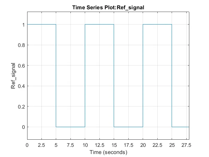
The reference signal is shown in the following figure.

Solution:-

The mass-spring-damper model consists of discrete mass nodes distributed throughout an object and interconnected via a network of springs and dampers. This model is well-suited for modeling objects with complex material properties such as nonlinearity and viscoelasticity. Packages such as MATLAB may be used to run simulations of such models. As well as engineering simulation, these systems have applications in computer graphics and computer animation.

The spring-mass-damper system consists of a mass with weight (m), a spring with stiffness (k), and a shock absorber with a damping coefficient of (c). This system works based on Newton’s second law, which states that Force is equal to the rate of change of momentum. For a constant mass, force equals mass times acceleration.

Deriving the Mass Spring Damper System based on Newton’s second law F = m*a

where

F = Resultant of all the forces

m = Mass

a = Acceleration

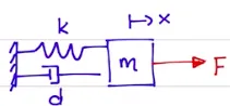
Fig1: Mass Spring Damper System in Rest

k is the spring stiffness

d is the damping coefficient

The above system is in a state of rest. Let's consider a moving Mass Spring Damper System to see forces act during motion. What are the forces acting if the system is moving?

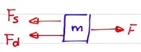
Fig2: Mass Spring Damper System in Motion

Expression for Spring Force and Damping Force

Fs = k*x ----(1)

Fd = d*(dx/dt) ----(2)

Applying F = m*a

ΣF = m*(d^2x/dt^2) (in the positive direction)

− Fs − Fd + F = m*(d^2x/dt^2)

F = m*(d^2x/dt^2) + Fd + Fs ----(3)

Substituting eq(1) and eq(2) in eq(3)

F = m*(d^2x/dt^2) + d*(dx/dt) + k*x

The above equation is the equation of motion (EOM).

Applying Laplace Transform to the above equation

F(s) = m*(s^2*x(s)) + d*(s*x(s)) + k*x(s)

F(s) = (m*s^2 + d*s + k)*x(s)

x(s)/F(s) = 1/(m*s^2 + d*s + k)......transfer fnc

The above equation is the transfer function

Model

The Simulink Model is built to obtain the transfer function of a mass spring damper system. A PID controller is also implemented into the system to adjust the force on the mass so that its position follows a reference signal.

Below are some of the block details used to create the Simulink Model,

Pulse Generator

(Generate square wave pulses at regular intervals)

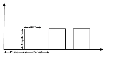
The Pulse Generator block generates square wave pulses at regular intervals. The block waveform parameters, Amplitude, Pulse Width, Period, and Phase delay, determine the shape of the output waveform. The following diagram shows how each parameter affects the waveform.

The suggested approach of the electromechanical damper mass spring control system will be subdivided into the following control models:

i)Control model with using PID controller unit

To maintain the required structure of the closed loop control system with using PID controller and unity feedback element, it is required to employ and calculate the following transfer functions

And (G₁, G₂ and G_C) can be expressed as follows:

G1=1(ms2+bs+k),(9)

G2=Vx,(10)

GC=(Kp+Kis+Kds),(11)

where

Taking G_T = (G_C)∗(G₁)∗(G₂)

Hence, the overall transfer function of the entire control system (G_sys) will be formed as follows [18]:

Gsys=GT(s)H(s)1+GT(s)H(s),(12)

With taking unity feedback H(s) = 1, then

Gsys=V(Kds2+Kps+Ki)x∗ms3+(x∗c+V∗Kd)s2+(V∗Kp+x∗k)s+V∗Ki,(13)

ii)Electromechanical Control system based on Backstepping Technique

The backstepping control design can be illustrated for the damper mass spring control system with applying the following steps [10–14]:

Step 1

The mathematical differential equation of the suggested damping system is given by:

d2xdt2+(bm)dxdt+(km)x=(1m)u,(14)

where (u) represents the external force.

The Eq. (14) can be rewritten as

m¨x=−kx−b˙x+u,(15)

Rearranging Eq. (15) as follows

¨x=−kmx−bm˙x+1mu,(16)

Hence

¨x=F(x)+g(t)u(t)+d(t),(17)

where:

The tracking error can be defined as follows:

e1=(xd−x),(18)

Then, the tracing error derivative can be represented as follows:

˙e1=(˙xd−˙x),(19)

The first Lyapunov function will be taken as follows:

V1=12eT1e1,(20)

And the derivative of the first Lyapunov function will become as

˙V1=eT1˙e1=eT1(˙xd−˙x),(21)

β=˙xd+k1e1,(22)

Where k₁ represents the positive constant.

If the virtual control is replaced with the desired value, then Eq. (21) becomes:

˙V1=−k1eT1e1≤0,(23)

And e2=(˙x−β).

Then e2=(˙x−˙xd−k1e1).

The sliding surface will be defined in terms of the error as:

s=e2=(˙x−β)=(˙x−˙xd−k1e1),(24)

Step 2

In this step of the backstepping control technique, the second Lyapunov function will be selected as follows [14–19]:

V2=V1+12sTs,(25)

And

˙V2=V1+12sT˙s,(26)

˙V2=eT1(−e2−λ1e1)+sT(F(x,t)+g(t)u(t)+d(t)−¨xd−k1˙e1,˙V2=eT1(−e2−λ1e1)+sT(F(x,t)+g(t)u(t)+d(t)−¨xd−k1˙e1,˙V2=−λ1eT1e1+sT(−e1+F(x,t)+g(t)u(t)+d(t)−¨xd−k1˙e1),(27)

Step 3

The external disturbance will be assumed as unknown, then the backstepping control scheme in final control signal can be obtained as follows:

u=1g(t)(−F(x,t)−k2s+e1+k1˙e1−¨xd),

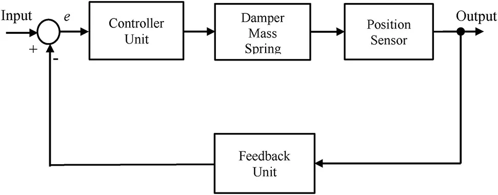
Schematic of a control system with TRAC in the adaptive outer loop

Fig (1)

Block diagram of an adaptive position control system for a spring-mass-damper system with a PI controller, full state feedback and TRAC in the adaptive outer loop

Square wave tracking of the system in Fig. 1 with the transfer functions in (15) for small (top) and large (bottom) parametric disturbances in the plant model

PID Controller

(Continuous-time or discrete-time PID controller)

This block implements continuous- and discrete-time PID control algorithms and includes advanced features such as anti-windup, external reset, and signal tracking. You can tune the PID gains automatically using the 'Tune...' button (requires Simulink Control Design).

Transfer Function

(Model linear system by transfer function)

The Transfer Fcn block models a linear system by a transfer function of the Laplace-domain variable s. The block can model single-input single-output (SISO) and single-input multiple-output (SIMO) systems.

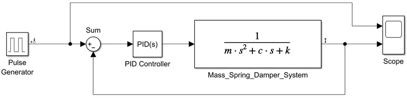
A Pulse Generator block is used as a reference Force input signal for the system. A Transfer function block is used for the implementation of the Mass Spring Damper system. The systems-derived equation in the Laplace transform is used in the transfer function. Variables of the same are defined through a Matlab script. The output of the transfer function is the displacement of the system, which is then fed back to the PID Controller as an error signal after subtracting it from the reference signal. Using a Controller the system throws the best tracking response.

Matlab Script

Variables m (mass), k (spring constant), and c (damping constant) used in the transfer function are defined through this Matlab script.

clear
clc
m = 3.6; % Mass [kg] 
k = 400; % Spring constant [N/m] 
c = 100; % Damping constant [Ns/m]

Pulse Generator

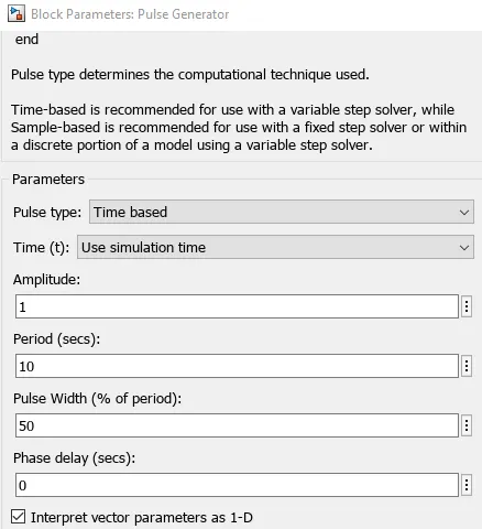
The parameters of the Pulse Generator are shown below. It satisfies the given reference signal for the system.

PID Controller

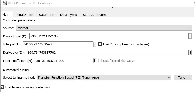
The PID values are selected automatically for the best response through PID Tuner.

PID Tuner

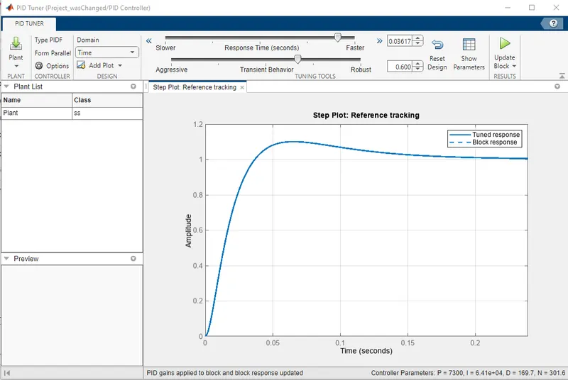
Below is the Tuned response of the PID Tuner. Response Time is increased manually for the best outcome and the same response is upgraded for the system using the Update Block option.

Scope Output

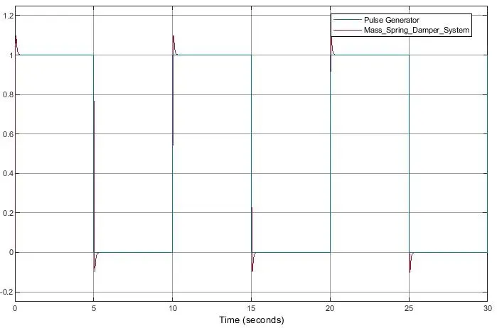
The Scope Output is the best tracking response of the system. It is achieved with the help of the PID Controller. Very small Overshoot and Undershoot of the signal can be seen.