Project - Position control of mass spring damper system

ANS:

OBJECTIVE:

• Obtain the transfer function of a mass spring damper system and use it in the model.

• Add a PID controller to adjust the force on mass so that its position follows a reference signal.

• Take m = 3.6kg / k = 400N/m / c = 100Ns/m

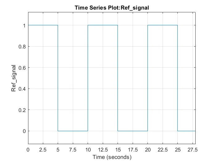
• The reference signal is shown in the following figure.

• 

MATLAB SCRIPT:

fig1

MATLAB SCRIPT EXPLANATION:

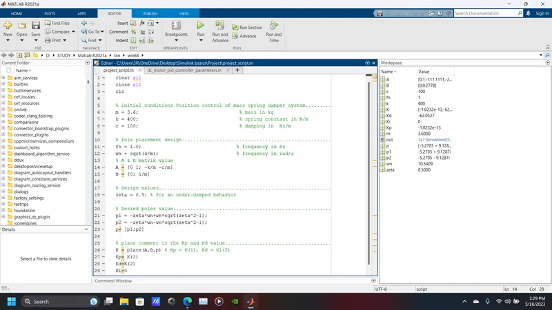
• The code initializes the position control of a mass-spring-damper system.
• System parameters are defined: mass (m), spring constant (k), and damping coefficient (c).
• Pole placement design is used to design the control system.
• The desired frequency (fn) and natural frequency (wn) are calculated based on the system parameters.
• The state-space matrices A and B are defined based on the system equations.
• Design values are set, including the desired damping ratio (zeta).
• The desired pole locations (p1 and p2) are calculated based on the desired frequency and damping ratio.
• The place function is used to calculate the control gains (K) based on the system matrices (A and B) and desired poles (p).
• The proportional gain (Kp), derivative gain (Kd), and integral gain (Ki) are extracted from the control gains (K).
• The integral gain (Ki) is set to 0.
• The code sets up a position control system for the mass-spring-damper system using the calculated control gains.

SIMULINK MODEL:

fig2

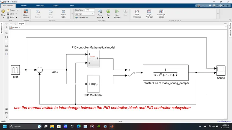
fig3

SIMULINK BLOCKS:

• gain
• sum
• integrator
• scope
• pulse generator
• transfer function
• pid controller
• manual switch

RESULTS:

fig4

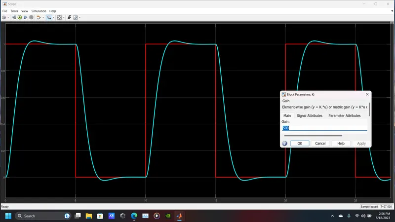
fig5

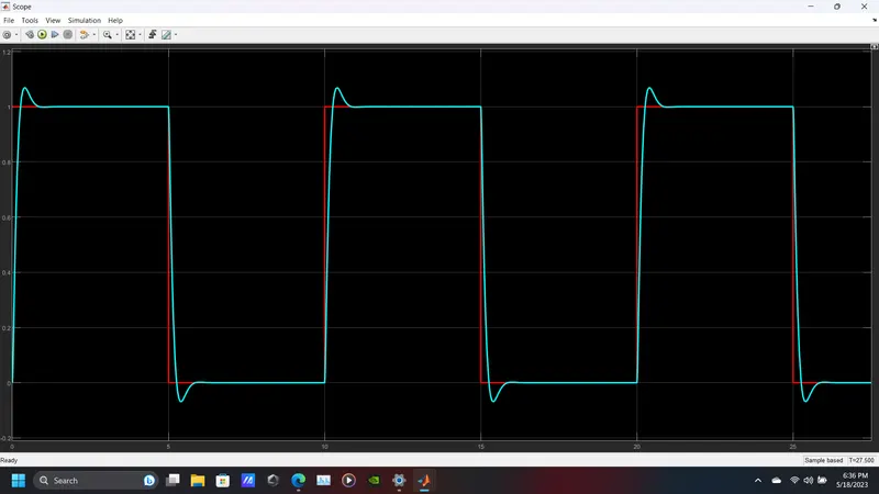
fig6

OBSERVATION:

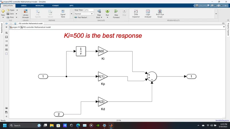
• Above shown simulink block is built using the Simulink blocks mentioned above. The model represents a mass, spring, and damper system using a PID controller.
• Use the Matlab code mentioned above. This code sets up a mass-spring-damper system and designs a position control using pole placement. The control gains (proportional, derivative, and integral) are determined based on the desired pole locations, damping ratio, and system parameters.
• First run the code and then run the model and observe the result.
• Observe the input in fig 4, which is a pulse wave of 50% pulse width with 10 secs with 1 amplitude. (marked in Red)
• In results in fig 4 it is observed that at Ki=500(after manually testing with several data which ranged from 0 to 10000) , the output gives the best response as an underdamped behaviour(zeta=0.5).(marked in Magenta)
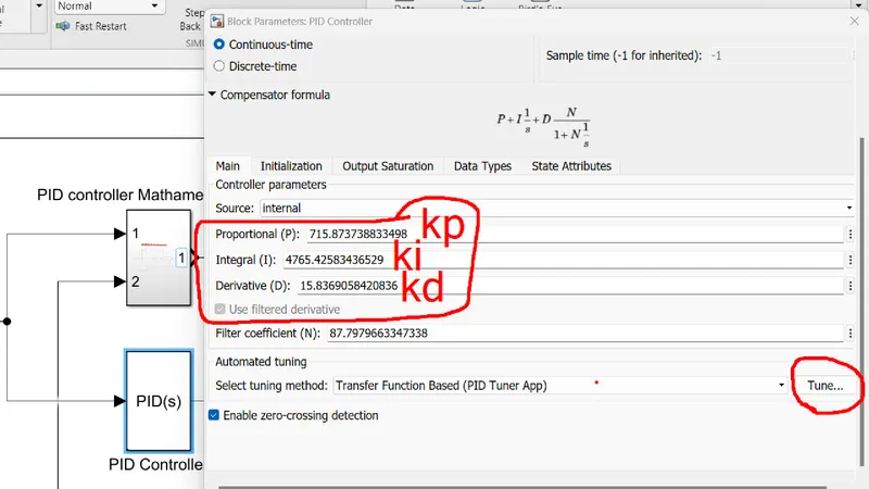
• In fig5 the best underdamped response can be observed, but it was done by tuning from the PID controller block shown in fig 6 where Kp=715.8736, Ki=4565.4258, and Kd=15.8360.
• The difference between using a PID controller ( done mathematically using sum,gain blocks) and inbuilt PID Controller block from the library is PID controller block derive the gain values like Kp, Ki, Kd first from the output for the best response and then adjust the parameters which are technically more accurate but when using the other method where Kp and Kd values are bound from the matlab code because you already defined the parameters as a result to get a best response one can only tune the value of Ki thus it is less accurate.