Project - Position control of mass spring damper system

CODES, MODELS & PARAMETERS

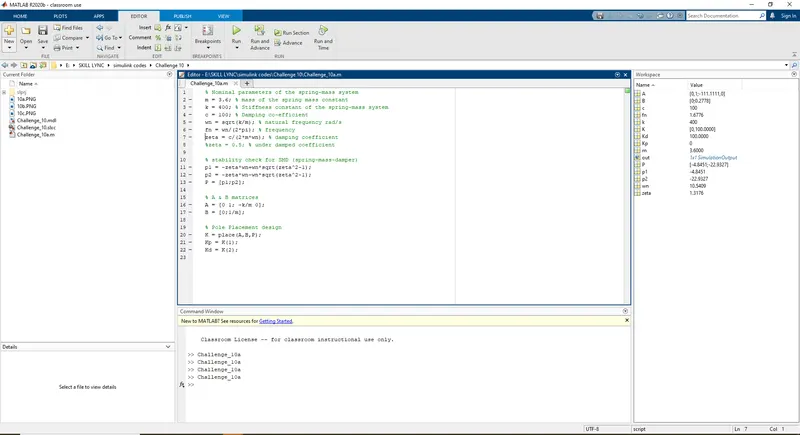
During the course of this project, the script that generates our parameters was first coded before the simulink model was designed.

Using the given variables m = 3.6, k = 400 and c = 100, the following variables were established.

Wn = 10.5409, fn = 1.6776, zeta = 1.3176, p1 = 4.8451, p2 = -22.9327, Kp = 100, Kd = 0.

the transfer function of the system was also deduced:

m`dx^2/dt`= f(t) - C`dx/dt`- kx

m*(s^2*x(s)) = F(s) - C*s*X(s) - kX(s)

x(s)/F(s) = 1/(ms^2 + cs + k)

x(s)/F(s) = 1/3.6s^2 + 100s + 400

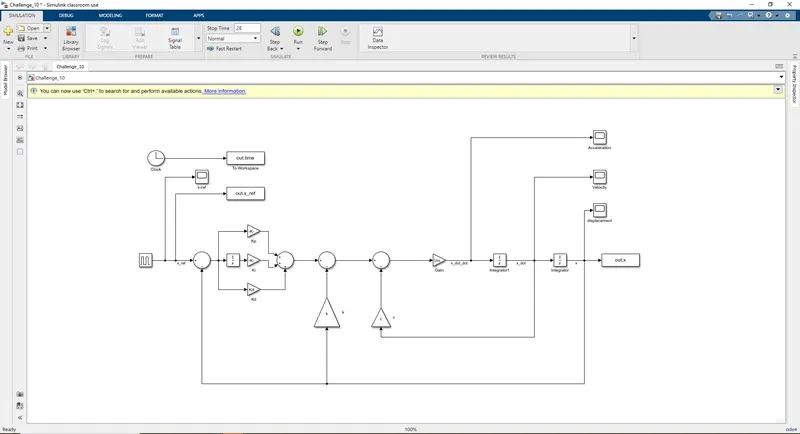
After these parameters were established, the simulink model was designed.

RESULTS & ANALYSIS

It is worth mentioning that the closed loop poles obtained using 'place' function was not sufficient to minimize the difference between of the output and the input signal. the default signal signal comparison is shown below.

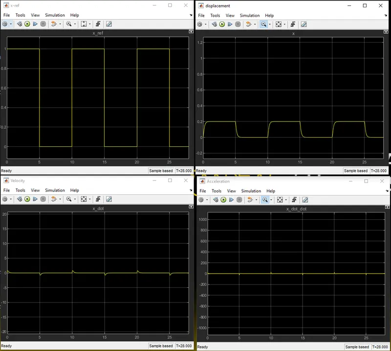
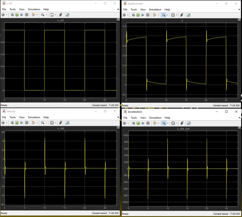
So iterations and adjustments were made to Kp, Ki & Kd until our goal of 10% overshoot, minimal steady error and optimal rise time was achieved. Our new K values are Kp = 3150, Ki = 1200, and Kd = 0.

DISPLACEMENT ANALYSIS

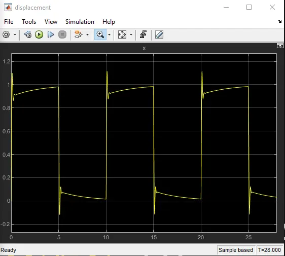
It was noticed that overshoots occurred at step times (5s,10s,15s,20s,25s). A steady state of 0.98 was achieved at the step times. A peak of 1.1 was attained whenever a pulse was exposed to the system and the minimum setting value was 0.861 was always attained. At step down times, the reverse resposne is generated which brings the signal to zero.These behaviours were repeated after every pulse/ step time through out the simulation.

VELOCITY ANALYSIS

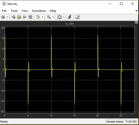
At step up times, the velocity signal rose to 16.625 units @ 0.0393s. Then it fell to -3.635 units @ 0.15s, it oscillated to 0.84 units @ 0.259s, Finally it reached a 0 m/s @ 0.3s and remains their until the next pulse. At step down times, the magnitude of the velocity is reversed to produce a mirrored signal along the x-axis.

ACCELERATION ANALYSIS

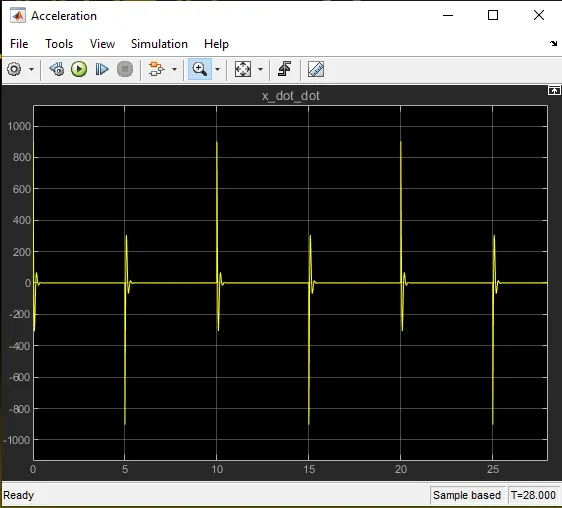
At step up times, the acceleration signal fell from 900 units @ 0s. Then it bottoms out to-306.65 units @ 0.078s, it oscillated up to 67.8 units @ 0.1881s, then it reached -15 m/s^2 @ 0.296s. After that the signal gets to 0 @ 0.4s and remains their until the next pulse. At step down times, the magnitude of the acceleration is reversed to produce a mirror signal across the x-axis.

CONCLUSION

The PID controller modeled the reference pulse signal as optimally as it could but at pulse/step times we noticed variations in terms of overshoot, oscillation, and delay in rise time. Kp, Ki and Kp can certainly be adjusted further to obtain better results.