Project - Position control of mass spring damper system

Position control of mass spring damper system:

AIM:

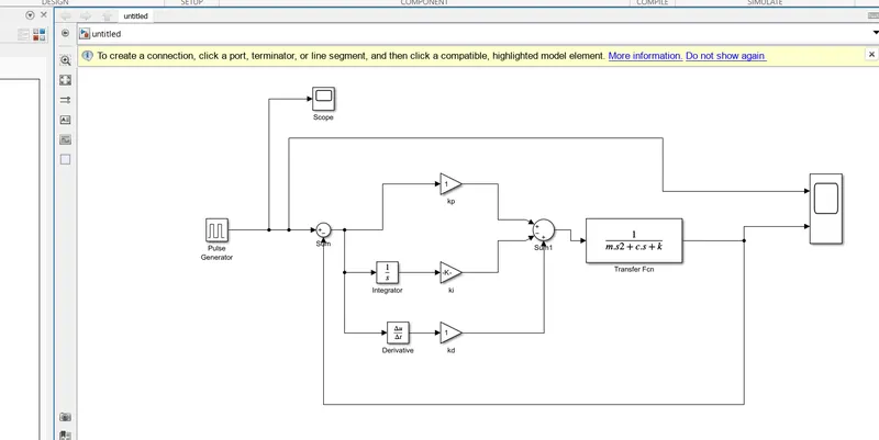
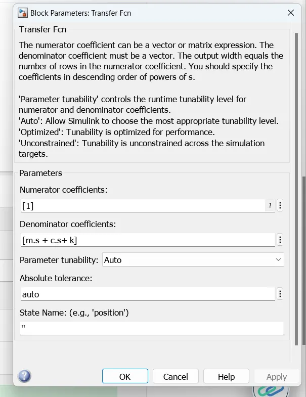
Obtain the transfer function of a mass spring damper system and use it in the model. Add a PID controller to adjust the force on mass so that its position follows a reference signal.

Take m = 3.6; %kg k = 400; %N/m c = 100; %Ns/m

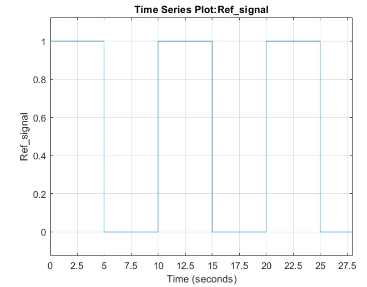
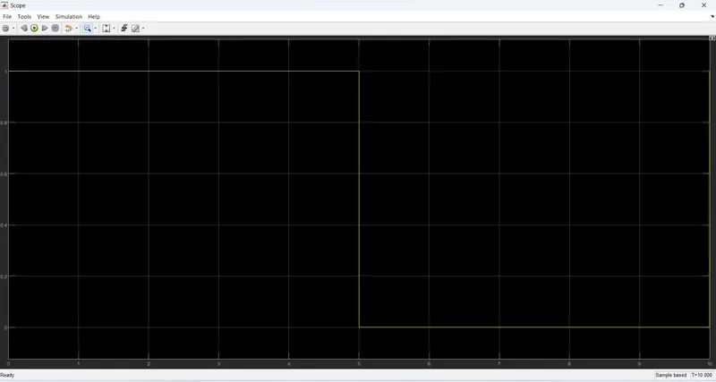
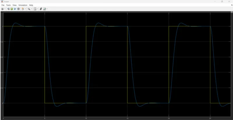
The reference signal is shown in the following figure.

Objective :

• Transfer function of a mass spring damper system and use it in the model. Add a PID controller to adjust the force on mass so that its position follows a reference signal. the matlab model of the pid control and transfer function pulse wavefrome generator.
• This example shows a controlled mass-spring-damper. A controller adjusts the force on the mass to have its position track a command signal. The initial velocity for the mass is 10 meters per second. The controller adjusts the force applied by the Force Source to track the step changes to the input signal.
• he mass-spring-damper model consists of discrete mass nodes distributed throughout an object and interconnected via a network of springs and dampers. This model is well-suited for modeling objects with complex material properties such as nonlinearity and viscoelasticity. Packages such as MATLAB may be used to run simulations of such models. As well as engineering simulation, these systems have applications in computer graphics and computer animation.
• The spring-mass-damper system consists of a mass with weight (m), a spring with stiffness (k), and a shock absorber with a damping coefficient of (c). This system works based on Newton’s second law, which states that Force is equal to the rate of change of momentum. For a constant mass, force equals mass times acceleration.
• Deriving the Mass Spring Damper System based on Newton’s second law F = m*a

where

F = Resultant of all the forces

m = Mass

a = Acceleration

PID controller

• A PID controller is an instrument used in industrial control applications to regulate temperature, flow, pressure, speed and other process variables. PID (proportional integral derivative) controllers use a control loop feedback mechanism to control process variables and are the most accurate and stable controller.
• A proportional–integral–derivative controller (PID controller or three-term controller) is a control loop mechanism employing feedback that is widely used in industrial control systems and a variety of other applications requiring continuously modulated control.
• PID control is a well-established way of driving a system towards a target position or level. It's a practically ubiquitous as a means of controlling temperature and finds application in myriad chemical and scientific processes as well as automation. PID control uses closed-loop control feedback to keep the actual output from a process as close to the target or setpoint output as possible.
• A digital PID controller reads the sensor signal, normally from a thermocouple or RTD and connects the measurement to engineering units, such as degree Fahrenheit or Celsius, that are then displayed in a digital format.
• We will now look at the effects of varying the Proportional component of the controller’s output, and of introducing Integral (I) and Derivative (V) terms.
• If we have just a Proportional (P) controller, we can start by setting the Kp gain to a modest value, such as 10 (K is dimensionless). After applying the step input, the output will be stable, but will approach the desired value slowly. If Kp is increased to, say, 100, both the steady state error and the rise time will be reduced – so far, so good. However, if we increase Kp to 200, although the rise time and steady state error are further reduced, overshoot starts to appear.
• From here on, further increasing Kp merely increases overshoot, with no further reductions in rise time or steady state error. And overshoot may eventually become underdamped oscillation, meaning that the system will be unstable.
• The industry’s solution to this has been to add Integral (I) and Derivative (V) components to the controller’s Proportional (P) output, to build a PID controller.

PID controller in this project

• In this project, PID controller has been designed by using Simulink in order to control a mass spring damper system which can move any direction. A transfer function for dc motor was added on the diagram. Response curve of the PID controller were fixed by tuning.
• The computer interface, different control algorithms can be performed on the system easily; control parameters can be set up online, filter algorithms in various structures can be tried and the reaction of these changeable values to the system can be observed.
• The effects of controller Proportional Integral Derivative (PID) for developing.

Spring Mass Damper

• Spring-mass-damper theory applies the basic physics of F=ma to define suspension motion and response on bump impacts. Force (F) acting on the suspension is the combination of spring plus damping force. Mass (m) is the chassis or wheel weight depending on which body you want to look at. The combination of force and mass define the F=ma acceleration, which in turn defines the velocity, position and suspension response characteristics at any instant in time.
• Spring force: Spring force is defined by the spring constant (k) multiplied by the displacement (dy)
• Mass: Mass of the wheel or mass of the chassis. Spring-mass-damper theory describes motion of either body
• Damping: The shock absorber damping coefficient defined as damping force divided by shaft velocity. Damping linearly increases with shaft velocity

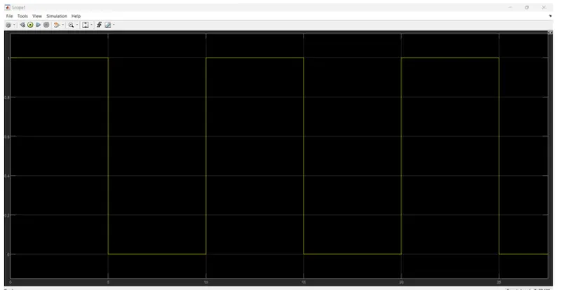
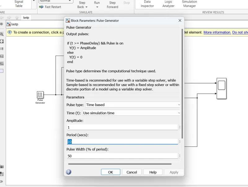
The block's Pulse type parameter allows you to specify whether the block's output is time-based or sample-based. If you select sample-based, the block computes its outputs at fixed intervals that you specify. If you select time-based, Simulink computes the block's outputs only at times when the output actually changes. This can result in fewer computations being required to compute the block's output over the simulation time period.

Depending on the pulse's waveform characteristics, the intervals between changes in the block's output can vary. For this reason, Simulink cannot use a fixed solver to compute the output of a time-based pulse generator. Simulink allows you to specify a fixed-step solver for models that contain time-based pulse generators. However, in this case, Simulink computes a fixed sample time for the time-based pulse generators. It then simulates the time-based pulse generators as sample-basedIf you select time-based as the block's pulse type, you must specify the pulse's phase delay and period in units of seconds.

If you specify sample-based, you must specify the block's sample time in seconds, using the Sample Time parameter, then specify the block's phase delay and period as integer multiples of the sample time. For example, suppose that you specify a sample time of 0.5 second. And suppose you want the pulse to repeat every two seconds. In this case, you would specify 4 as the value of the block's Period parameter

Data Type Support:

A Pulse Generator block outputs real signals of any data type except int64 and uint64. The data type of the output signal is the same as that of the Amplitude parameter.

Pulse type:The pulse type for this block: time-based or sample-based. The default is time-based.

Amplitude:The pulse amplitude. The default is 1.

Period:The pulse period specified in seconds if the pulse type is time-based or as number of sample times if the pulse type is sample-based. The default is 2.

Pulse width:The duty cycle specified as the percentage of the pulse period that the signal is on if time-based or as number of sample times if sample-based. The default is 50 percent.

Phase delay:The delay before the pulse is generated specified in seconds if the pulse type is time-based or as number of sample times if the pulse type is sample-based. The default is 0 seconds.

Sample Time:The length of the sample time for this block in seconds. This parameter appears only if the block's pulse type is sample-based. See Specifying Sample Time for more information.

Interpret vector parameters as 1-D:If this option is selected and the other parameters are one-row or one-column matrices, after scalar expansion, the block outputs a 1-D signal (vector). Otherwise the output dimensionality is the same as that of the other parameters.

The Sum block performs addition or subtraction on its inputs. This block can add or subtract scalar, vector, or matrix inputs. It can also collapse the elements of a single input vector.

You specify the operations of the block with the List of Signs parameter. Plus (+), minus (-), and spacer (|) characters indicate the operations to be performed on the inputs:

• If there are two or more inputs, then the number of characters must equal the number of inputs. For example, "+-+" requires three inputs and configures the block to subtract the second (middle) input from the first (top) input, and then add the third (bottom) input.

• All nonscalar inputs must have the same dimensions. Scalar inputs will be expanded to have the same dimensions as the other inputs.

• A spacer character creates extra space between ports on the block's icon.
• If only addition of all inputs is required, then a numeric parameter value equal to the number of inputs can be supplied instead of "+" characters.
• if only one vector is input, then a single "+" or "-" will collapse the vector using the specified operation.

When the Show additional parameters check box is selected, some of the parameters that become visible are common to many blocks. For a detailed description of these parameters, refer to Block Parameters in the Fixed-Point Blockset documentation.

Data Type Support:

The Sum block accepts signals of any complexity and data type, including fixed-point data types, except int64 and uint64. The inputs may be of different data types unless the Require all inputs to have same data type parameter is selected.

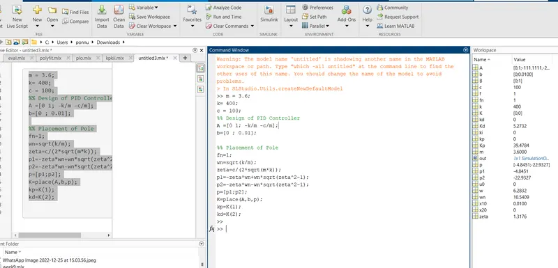
code

m = 3.6;
k= 400;
c = 100;
%% Design of PID Controller
A =[0 1; -k/m -c/m];
b=[0 ; 0.01];

%% Placement of Pole
fn=1;
wn=sqrt(k/m);
zeta=c/(2*sqrt(m*k));
p1=-zeta*wn+wn*sqrt(zeta^2-1);
p2=-zeta*wn-wn*sqrt(zeta^2-1);
p=[p1;p2];
K=place(A,b,p);
kp=K(1);
kd=K(2);

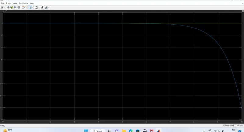
CONCLUSION :

To complte the project of Position control of mass spring damper system transfer function of a mass spring damper system and use it in the model. Add a PID controller to adjust the force on mass so that its position follows a reference signal to using matlab and simulink wave from plot.