Project 9

Object tracking:

• Object tracking is the process of identifying and following an object as it moves in a video. The object can be anything that appears in the video, such as a person, a car, or a ball. Object tracking involves detecting the object in each frame of the video and then predicting its position in future frames based on its past movements. This can be useful in a variety of applications, such as video surveillance, robotics, and autonomous vehicles.
• More technically, object tracking is an application of deep learning where the program takes the initial set of detections, assigns the unique identifications for each of the initial detections, and then tracks the detected objects as they move around frames in the video.
• This can be especially challenging when the objects move in complex ways, such as changing perspectives or overlapping with each other.
• there are two levels of tracking
• Single object tracking (SOT)
• In this type of tracking, the tracker tracks only a single object even if there are many objects present in the frame. This method of tracking is very fast and easier.
• In this, there are some traditional trackers used for tracking like CSRT, and KCF. However deep learning-based trackers are now proven to be far more accurate than traditional trackers. For example SiamRPN and GOTURN
• Multiple object tracking (MOT)
• In this type of tracking, trackers track multiple objects present in a frame. Multiple object trackers are trained on a large amount of data, unlike traditional trackers. Therefore, they are proven more accurate as they can track multiple objects and even different classes at the same time while maintaining high speed.
• In this, there are some powerful algorithms like DeepSort, JDE, and CenterTrack are used for tracking multiple objects in this frame.

SORT & DeepSort

• DeepSort is the most popular and one of the most widely used, elegant object-tracking algorithms. It is an extension of SORT(Simple Real-time Tracker).
• DeepSORT introduces deep learning into the SORT algorithm by adding an appearance descriptor to reduce identity switches, Hence making tracking more efficient.
• let's first understand the SORT algorithm
• Simple Online Real Time Tracking(SORT)
• SORT is an approach to Object tracking where rudimentary approaches like Kalman filters and Hungarian algorithms are used to track objects and claim to be better than many online trackers. SORT is made of 4 key components which are as follows.
• Detection:
• This is the first step in the tracking module. In this step, object detectors like FrRCNN, and YOLO are used to detect the objects in the frame that are to be tracked. These detections are then passed on to the next step.
• Estimation:
• In multiple object tracking, the estimation step is an important part of the process of following objects as they move through a video. During this step, we try to predict the future position of each target object based on its current position and velocity. To do this, we use a constant velocity model, which assumes that the object will move at a constant speed and in a straight line between frames.
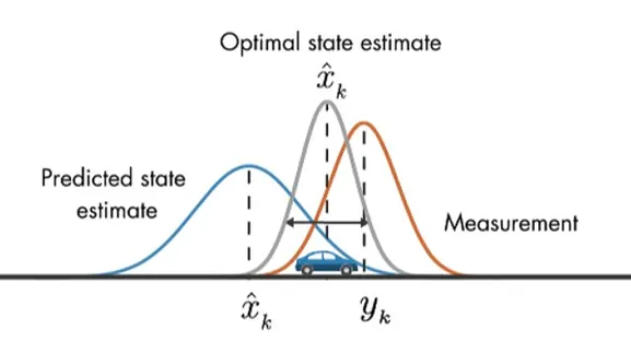
• However, real-world observations of the target object can be noisy and uncertain, which can make it difficult to accurately predict its future position. To address this issue, we use a Kalman filter to help refine our prediction. A Kalman filter is a type of recursive Bayesian filter that can estimate the state of a system (in this case, the position and velocity of the target object) based on noisy and uncertain observations.
• At each time step, it receives an observation of the target object and uses it to update its estimate of the object's position and velocity. This helps to refine the prediction and improve its accuracy, allowing us to track the movement of the object.
• Data association:
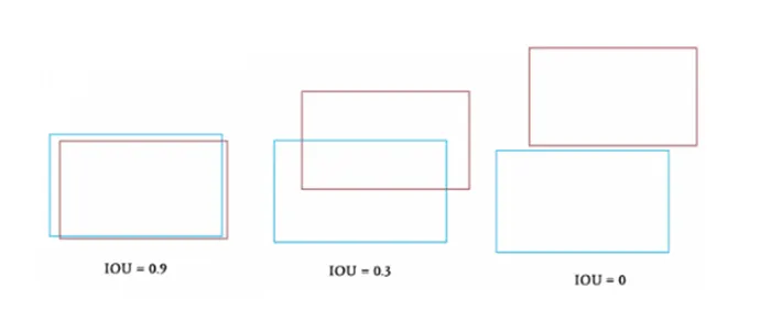
• When we have a detected bounding box and a target bounding box, we want to determine whether the detection corresponds to the target or if it represents a new object. To do this, we compute a cost matrix that reflects the similarity between the detection and each of the predicted bounding boxes of the existing targets. One way to measure this similarity is by using the intersection-over-union (IOU) distance, which is a metric that calculates the overlap between two bounding boxes and normalizes it by the union of the boxes.
• Once we have the cost matrix, we can use the Hungarian algorithm to find the optimal assignment of detections to targets. This algorithm finds the minimum-cost assignment of a set of rows to a set of columns, given a cost matrix. In our case, the rows correspond to the detections and the columns correspond to the predicted bounding boxes of the existing targets.
• However, sometimes a detection may not correspond to any of the existing targets, or the similarity between a detection and a target may be too low to consider them as a match. To handle these cases, we use a threshold value called IOUmin. If the IOU of detection and a target is less than IOUmin, then we reject that assignment and consider the detection as a new object.
• Creation and Deletion of Track Identities:
• This module is responsible for the creation and deletion of track IDs as follows
• When a new object is detected, it is given a unique ID to help track it over time.
• If the detected object is not similar enough to any of the existing targets (as measured by the IOUmin threshold), it is treated as a new object and given a new ID.
• If an object has not been detected for a certain number of frames (called TLost), its ID is deleted because it is assumed to no longer be present in the scene.
• If the object reappears after being lost, it will be treated as a new object and given a new ID. The tracking will resume automatically under the new identity.
• The process of creating and deleting IDs helps to accurately track objects and associate them with their corresponding bounding boxes.
• Deep Simple online Real-time tracking(DeepSort)
• DeepSort is an object-tracking algorithm that was designed to improve upon the performance of SORT, a popular object-tracking algorithm that uses Kalman filters and the Hungarian algorithm. One of the main limitations of SORT is that it tends to produce a relatively high number of identity switches, especially when tracking objects that are occluded or viewed from different viewpoints.
• To address this issue, the authors of DeepSort introduced a deep learning component to the algorithm. This component allows DeepSort to extract visual features from the objects being tracked, which are used to compute a distance metric based on the "appearance" of the object. This helps to reduce the number of identity switches and improve the accuracy of tracking.
• To implement DeepSort, the following steps are followed:
• Object detection: The object detection component of DeepSort uses an object detector, such as FrRCNN or YOLO, to detect objects in the frame and return their bounding boxes.
• Hungarian Algorithm: The Hungarian algorithm, also known as the Kuhn-Munkres algorithm, is a method for assigning IDs to objects that have been detected in a video or image. It uses a scoring metric to determine the best match for each object and helps to accurately track the movements of the objects over time.
• There are three main types of scoring metrics that can be used: Intersection over union (IoU), shape score, and convolution cost.
• For example, When have two lists of boxes from YOLO: one from the previous frame (t -1) and another from the current frame List(t). The Hungarian Algorithm goes through these lists and calculates a score for each bounding box based on how much they overlap.
• The more overlap there is, the higher the score will be. This score is then used to determine which detections should be associated with which tracked objects.
• 

Kalman filters:

• The Kalman filter is a mathematical method used to predict the future position of an object based on its current position and velocity.
• It is commonly used in object tracking applications to smooth out noisy measurements and reduce the risk of identity switches due to large movements. By accounting for statistical noise in the measurements, the Kalman filter is able to accurately predict the future position of the object and improve the accuracy of tracking.
• 

Estimating Bounding Box State with a Kalman Filter

• The main objective of using a Kalman filter for bounding box tracking is to estimate the state of the bounding box, which includes the mean (e.g., the coordinates of the bounding box) and the covariance (i.e., the uncertainty in the bounding box's state).
• The mean of the bounding box's state is represented by a state vector, which might include the center coordinates`[Cx, Cy]`, size`[w,h]`, and velocity`[Vx, Vy, Vw, Vh]` of the bounding box.
• state vector `X = [Cx, Cy,w,h, Vx, Vy, Vw, Vh]`
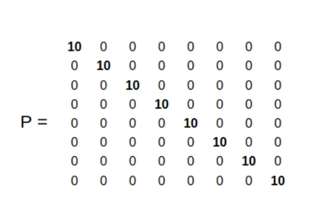
• The covariance matrix represents the uncertainty in the bounding box's state. In general, a larger value for the covariance matrix indicates a greater uncertainty in the bounding box's state.
• For example, if the covariance matrix has large values for the position elements (e.g., the center coordinates of the bounding box), it means that there is high uncertainty in the bounding box's position. This could be due to a variety of factors, such as noise in the measurements or significant changes in the bounding box's motion.
• It is common to set the initial values of the covariance matrix to arbitrary numbers and then adjust them over time based on the measurements made of the bounding box.
• 
• The Kalman filter works in two steps: prediction and update.
• Prediction Step
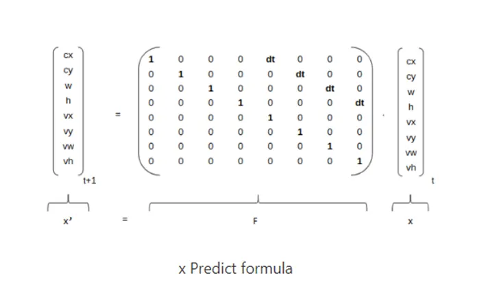
• In the prediction step, the Kalman filter uses the state transition model to predict the next state of the bounding box based on its current state and any control inputs (e.g., external forces acting on the object). This prediction is based on the past motion of the bounding box and produces an estimate of its future location.
• predicted_state (x')= state_transition_model(F) * current_state(x) + control_input(u)
• `x' = Fx +u`
• `P' = FPF^T + Q`
• Note:control_input(u) is a vector that represents any external forces acting on the bounding box, here we are not using it.
• 
• Update step
• The update phase is a correction step. It includes the new measurement (z) and helps improve our filter.
• The process of update is to start by measuring an error between measurement (z) and predicted mean.
• `y = z-Hx'` , y = error
• `S = HP'H^T + R` , H = measurement matrix , R = measurement noise , P' = predicted estimate of the state covariance
• The second step is to calculate a Kalman Gain (K)
• `K = P'H^TS^(-1)` , K = Kalman Gain
• The Kalman gain is used to estimate the importance of our error. We use it as a multiplication factor in the final formula to estimate a new x.
• `x = x'+ Ky` , x = new measurement`
• If the Kalman gain is large, it means that the new measurement is highly reliable and should be given more weight in the update. If the Kalman gain is small, it means that the new measurement is less reliable and should be given less weight in the update.
• `P= (I - K*H) * P'`, P = uncertainty in the estimate of the system's state, `I`= identity matrix
• Let us move to the Implementation of deep sort

Implementation

• As We know, the Deep Sort algorithm used for tracking objects in a video stream relies on the output of the object detection model as its input. In this project, we have used the YOLOv3 version of YOLO for detection.
• Here is my Project GitHub Repo: Object detection and tracking
• Here is my project directory
• 
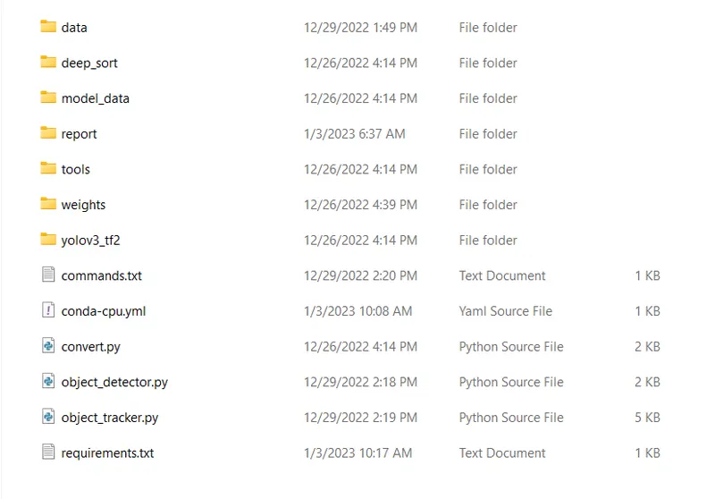
• The conda-cpu.yml file is used to set up an environment for the project and requirements.txt is to install the dependencies as follows
• 1. Create Environment (Conda recommended)
  #Tensorflow CPU
  conda env create -f conda-cpu.yml
  conda activate tracker-cpu
• 2. Install dependencies
  #Tensorflow CPU
  pip install -r requirements.txt
• The 'data' folder contains the font, labels, and test video
• The 'yolov3_tf2' folder contains
• 
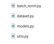
• 'weights' folder contains the pre-trained Darknet Yolov3 weights file which is directly downloaded from https://pjreddie.com/media/files/yolov3.weights
• 
• 'convert.py' used to convert weights from yolov3.weight to yolov3.tf format and Use the python convert.py command for conversion.
• 'tool' contains the following files
• 
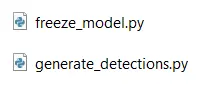
• The 'deepsort' folder contains the following and which responsible for tracking objects.
• 

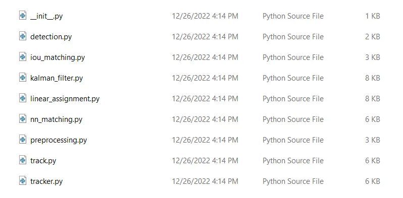
Till now we have done most of the work

Now it's time to track the vehicles in the video stream and in order to accomplish this we will be using the object_tracker.py file.

object_tracker.py

# Importing libraries
from absl import flags #
import sys
FLAGS = flags.FLAGS
FLAGS(sys.argv)

import time        # used to measure time taken by block
import numpy as np # used to perform mathematical operation 
import cv2         # used for reading,writing,displying and manupulating the image
import matplotlib.pyplot as plt #used to visvulize the results 

import tensorflow as tf
#importing function from custom modules inside yolov3_tf2 which are necessary for detection 
from yolov3_tf2.models import YoloV3
from yolov3_tf2.dataset import transform_images
from yolov3_tf2.utils import convert_boxes
# importing custom modules and functions from deep_sort,which are necessary for tracking task
from deep_sort import preprocessing
from deep_sort import nn_matching
from deep_sort.detection import Detection
from deep_sort.tracker import Tracker
from tools import generate_detections as gdet

class_names = [c.strip() for c in open('./data/labels/coco.names').readlines()] # list of class names created by reading names from coco.nmaes files
yolo = YoloV3(classes=len(class_names))    # creating yolo model
yolo.load_weights('./weights/yolov3.tf')   # loading pre-trained .tf weight from weights folder

# defining the parametrs
max_cosine_distance = 0.4
nn_budget = None
nms_max_overlap = 0.6

# Initialize deep sort objects
model_filename = 'model_data/mars-small128.pb'
# setting up encoder for feature extraction from image.
encoder = gdet.create_box_encoder(model_filename, batch_size=1)
# claculate cosine distance metric
metric = nn_matching.NearestNeighborDistanceMetric('cosine', max_cosine_distance, nn_budget)
# Initilizing deepsort tracker
tracker = Tracker(metric) 

vid = cv2.VideoCapture('./data/video/traffic.mp4') # capturing frames from video

codec = cv2.VideoWriter_fourcc(*'XVID') # codec format used while writing video file
vid_fps =int(vid.get(cv2.CAP_PROP_FPS)) # frame per second used while writing
vid_width,vid_height = int(vid.get(cv2.CAP_PROP_FRAME_WIDTH)), int(vid.get(cv2.CAP_PROP_FRAME_HEIGHT)) #size of frame in vide
out = cv2.VideoWriter('./data/video/results.avi', codec, vid_fps, (vid_width, vid_height)) #writing frame to file

from _collections import deque
pts = [deque(maxlen=30) for _ in range(1000)] #

#counter = []
cv2.namedWindow("output", cv2.WINDOW_NORMAL)
while True:
    _, img = vid.read()
    if img is None:
        print('Completed')
        break

    img_in = cv2.cvtColor(img, cv2.COLOR_BGR2RGB) # convert BGR to RGB
    img_in = tf.expand_dims(img_in, 0)   # expanding dimensions by adding extra dimenion to image tensor
    img_in = transform_images(img_in, 416) # image transformation 

    t1 = time.time() # start time 

    boxes, scores, classes, nums = yolo.predict(img_in) # detection using yolov3

    classes = classes[0] # class label
    names = []
    for i in range(len(classes)):
        names.append(class_names[int(classes[i])])
    names = np.array(names)
    converted_boxes = convert_boxes(img, boxes[0]) # convert bounding box to required format
    features = encoder(img, converted_boxes)  # extract features
    
    # storing required imformation in list
    detections = [Detection(bbox, score, class_name, feature) for bbox, score, class_name, feature in
                  zip(converted_boxes, scores[0], names, features)]
    
    # extract bounding boxes,scores and class labels from detection list
    boxs = np.array([d.tlwh for d in detections])
    scores = np.array([d.confidence for d in detections])
    classes = np.array([d.class_name for d in detections])
    # apply non_max_suppression to the detections
    indices = preprocessing.non_max_suppression(boxs, classes, nms_max_overlap, scores)
    detections = [detections[i] for i in indices]
    
    # call tracker
    tracker.predict() 
    tracker.update(detections)

    # color map
    cmap = plt.get_cmap('tab20b') # colormap created
    colors = [cmap(i)[:3] for i in np.linspace(0,1,20)] # list of color generated from colormap
    
    # iterate over the tracks in tracker
    for track in tracker.tracks:
        if not track.is_confirmed() or track.time_since_update >1: # skip the track if condition not meet
            continue
        bbox = track.to_tlbr() # convert the tracks bounding box
        class_name= track.get_class() # get class labels of track
        color = colors[int(track.track_id) % len(colors)] # color selection based on track ID's
        color = [i * 255 for i in color]   #scaling color from range 0 -1 to range 0-255
        
        # drawing bounding box rectanges and class name and track id
        cv2.rectangle(img, (int(bbox[0]),int(bbox[1])), (int(bbox[2]),int(bbox[3])), color, 2)
        cv2.rectangle(img, (int(bbox[0]), int(bbox[1]-30)), (int(bbox[0])+(len(class_name)
                    +len(str(track.track_id)))*12, int(bbox[1])), color, -1)
        cv2.putText(img, class_name+"-"+str(track.track_id), (int(bbox[0]), int(bbox[1]-10)), 0, 0.5,
                    (255, 255, 255),2)
        
        # calculate the center of bounding box for drawing tracking lines on image
        center = (int(((bbox[0]) + (bbox[2]))/2), int(((bbox[1])+(bbox[3]))/2))
        pts[track.track_id].append(center)
        
        # Iterate through the list of center points for the track
        for j in range(1, len(pts[track.track_id])):
            if pts[track.track_id][j-1] is None or pts[track.track_id][j] is None:
                continue
            # calculate the thickness of lines
            thickness = int(np.sqrt(64/float(j+1))*2)
            # draw line on the image connecting two center points
            cv2.line(img, (pts[track.track_id][j-1]), (pts[track.track_id][j]), color, thickness)


    fps = 1./(time.time()-t1)
    cv2.putText(img, "FPS: {:.2f}".format(fps), (0,30), 0,0.5,(0,0,255),2) 
    cv2.resizeWindow('output', 1024, 768)
    cv2.imshow('output', img)
    out.write(img)

    if cv2.waitKey(1) == ord('q'): #
        break
vid.release() # release video capture object
out.release() # release video writer object
cv2.destroyAllWindows() # destroy all windows

Here is the detailed explanation of object_tracker.py

Importing flags module from absl library

# Importing libraries
from absl import flags #
import sys
FLAGS = flags.FLAGS
FLAGS(sys.argv)

import time        # used to measure the time taken by block
import numpy as np # used to perform a mathematical operation 
import cv2         # used for reading, writing, displaying, and manipulating the image
import matplotlib.pyplot as plt #used to visualize the results 

Importing tensorflow and other custom modules and functions from yolov3_tf2 and deep_sort.

import tensorflow as tf
#importing function from custom modules inside yolov3_tf2 which are necessary for detection 
from yolov3_tf2.models import YoloV3
from yolov3_tf2.dataset import transform_images
from yolov3_tf2.utils import convert_boxes
# importing custom modules and functions from deep_sort,which are necessary for tracking task
from deep_sort import preprocessing
from deep_sort import nn_matching
from deep_sort.detection import Detection
from deep_sort.tracker import Tracker
from tools import generate_detections as gdet

class_names = [c.strip() for c in open('./data/labels/coco.names').readlines()] # list of class names created by reading names from coco.names files
yolo = YoloV3(classes=len(class_names))    # creating yolo model
yolo.load_weights('./weights/yolov3.tf')   # loading pre-trained .tf weight from weights folder

• The first line of code creates a list of class names by reading names from coco. names file which is stored .data/labels/
• Then line code creates the yolo model and stores it in the yolo variable and then loads weights from the weights folder.

# defining the parameters
max_cosine_distance = 0.5
nn_budget = None
nms_max_overlap = 0.8

• The above code defines the object tracking parameters.
• The'max_cosine_distance' is the maximum cosine distance for the nearest neighbor distance metric, which is used to compare the features of detections to determine if they correspond to the same object.
• The 'nn_budget' is the maximum size of the list of nearest neighbors that the distance metric keeps a track of. and if it is set equal to None it means a list has no size limit.
• The'nms_max_overlap' used as threshold in nms_max_suppresion and it specifies maximum overlap that is allowed between two bounding boxes before one of boxes is eliminated.

# Initialize deep sort object
model_filename = 'model_data/mars-small128.pb'
# setting up encoder for feature extraction from image
encoder = gdet.create_box_encoder(model_filename, batch_size=1)

• In the above code, we set up an encoder which is a pre-trained model for feature extraction from images.
• create_box_encoder() function creates an encoder object that can be used to extract features from a batch of images and bounding boxes.
• It takes two arguments one is 'model_filename' and the second one is 'batch_size'
• 'batch_size = 1' means the encoder passes one image and one bounding box at a time.

# calculate cosine distance metric
metric = nn_matching.NearestNeighborDistanceMetric('cosine', max_cosine_distance, nn_budget)

• In the above code, the 'metric' object is created using 'NearestNeighbhorDistanceMetric' from the 'nn_matching' module.
• 'NearestNeighbhorDistanceMetric'class takes three arguments metric,matching_threshold, and nn_budget.
• In this, we set the distance metric as 'cosine', and matching_threshold = max_cosine_distance
• the metric is used to calculate the similarity between pairs of feature vectors using a cosine distance metric.

# Initializing deepsort tracker
tracker = Tracker(metric)

• In the above code, we initialize the deepsort tracker by passing the above 'metric'.
• tracker object is created by calling the 'Tracker class' with the 'metric' argument.

vid = cv2.VideoCapture('./data/video/traffic.mp4') #used to capture frames from the video

• The 'vid' object is created by calling the 'cv2.VideoCapture()' function and it takes video_path as an argument.
• The 'VideoCapture'class is a class from the 'cv2'library and is used to capture the frames from a video file or camera.
• It has several methods that can be used to read and manipulate the video, such as 'read()',' get()', and release()'.

codec = cv2.VideoWriter_fourcc(*'XVID') #codec format that is to be used while writing video files.

• codec is an integer value used while writing a video and it is created by calling the 'cv2.VideoWriter_fourcc()' function.

vid_fps =int(vid.get(cv2.CAP_PROP_FPS)) # frame per second used while writing video file
vid_width,vid_height = int(vid.get(cv2.CAP_PROP_FRAME_WIDTH)), int(vid.get(cv2.CAP_PROP_FRAME_HEIGHT)) #size of frame in video

• vid_fsp is the frame rate of the video and it is obtained by calling the get'()' method of the 'vid' object by passing the 'cv2.CAP_PROP_FRAME_WIDTH' argument.
• 'vid_width', and 'vid_height'is the size of the video frame, and these are obtained by calling the 'get()' method of the 'vid' object with 'cv2.CAP_PROP_FRAME_WIDTH' and 'cv2.CAP_PROP_FRAME_HEIGHT' respectively.
• These variables are used while writing video files.

out = cv2.VideoWriter('./data/video/results.avi',codec,vid_fps,(vid_width, vid_height))# used to write frame to file

• In the above line of code, 'out' is an object created by calling the 'cv2.VideoWriter()' function of the 'cv2' library and used to write video frames to file.
• It takes four arguments such as 'path to the output file', 'codec', 'frame rate', and 'size'

#importing deque 
from _collections import deque #deque means 'double-ended queue'
pts = [deque(maxlen=30) for _ in range(1000)] 

• importing deque
• 'deque' means 'double-ended queue' which means we can add or remove elements from either end.
• The 'pts' list is used to track the paths of up to 1000 objects in the video.
• Each path is stored in a 'deque', which allows us to add or remove elements from either end.
• The 'deque' has a maximum size of 30 elements, which means that we can store the path of each object for up to 30 frames.
• The path of an object is tracked by storing the bounding box (BBox) of the object.
• When the number of frames exceeds 30, the oldest bounding box (BBox) of the object is automatically removed from the deque to make room for a new BBox.

#The 'While True' loop will cause the code to keep reading and processing frames 
while True:
    _, img = vid.read() #read frames from video capture object
    if img is None:     
        print('Completed')
        break

• The above code reads an image from the video capture object using the read() method.
• read() method returns a tuple containing a boolean value and image and when the boolean value is True the image read correctly and if the boolean value is False there image could not be read.
• checking if the image is None then print('completed') and break the loop.

    img_in = cv2.cvtColor(img, cv2.COLOR_BGR2RGB) #converting image BGR to RGB
    img_in = tf.expand_dims(img_in, 0)            #Adding an extra dimension to the image tensor
    img_in = transform_images(img_in, 416)        #applying image transformation

• The first line of code converts the image from BGR to RGB using OpenCV 'cv2.COLOR_BGR2RGB' function
• In the second line of code add an extra dimension to the image tensor using tensorflow 'tf.expand_dims' function.
• This is because our input image has the shape of (height, width, channels) but the Convolutional Neural network expects the image into this shape (batch_size, height, width, channels).
• By adding extra dimension using 'tf.expand_dims(img_in,0) shape becomes (1, height, width, channels).
• This allows the CNN to process the image as a batch of size 1, rather than as a single image.

    t1 = time.time() #current time
    boxes, scores, classes, nums = yolo.predict(img_in) #detection using yolov3   

• This line of code uses predict() method to perform object detection using yolo model
• It takes the input image as an argument, performs detections, and returns a tuple of four values:'boxes', 'scores', 'classes', and 'nums'.
• 'boxes',= [(xmin1, ymin1, xmax1, ymax1), (xmin2, ymin2, xmax2, ymax2).......(xminN, yminN, xmaxN, ymaxN)]
• 'scores', = [score1,score2....scoreN]
• 'classes', = [class1, class2,.....classsN]
• 'nums' = Number of detection = len(boxes)

    classes = classes[0] # class label for first detection
    names = []           # empty list 
    # loop over class labels 
    for i in range(len(classes)):
        names.append(class_names[int(classes[i])]) # appending corresponding class names 
    names = np.array(names)                        # list to numpy array

• Above code, classes[0] extract the class labels for the first detection, loop over the class labels, and append corresponding class names
• convert the name list to numpy array.

    converted_boxes = convert_boxes(img, boxes[0]) # convert bounding box to required format
    features = encoder(img, converted_boxes) # extract features

• The first line of code convert bounding boxes for the first detection to the format that can be used with the feature extractor.
• The second line of code extracts the feature vectors for the detected objects using the encoder

     # storing required information in list
     detections = [Detection(bbox, score, class_name, feature) for bbox, score, class_name, feature in
                  zip(converted_boxes, scores[0], names, features)]

• The above code creates a list of Detection objects by zipping together the converted bounding boxes, scores,class_names, and features.

    # Extract boxs, scores, and class labels from detection list
    boxs = np.array([d.tlwh for d in detections]) 
    scores = np.array([d.confidence for d in detections])
    classes = np.array([d.class_name for d in detections])

    # Apply non_max suppression to the detections
    indices = preprocessing.non_max_suppression(boxs, classes, nms_max_overlap, scores)
    detections = [detections[i] for i in indices]

• The above code first extracts the bounding boxes,class labels, and confidence score from the detection list into separate arrays.
• Then apply non_max_suppression to these detection
• preprocessing.non_max_suppression() function takes boxs,scores,classes and nms_max_overlap as arguments and returns a list of indices of bounding boxes that should be kept after nms.
• then at last line of code create a detection list.

    # color map
    cmap = plt.get_cmap('tab20b') #colormap is created
    colors = [cmap(i)[:3] for i in np.linspace(0,1,20)] # list of color generated from colormap

• In first line of code colormap is created using 'plt.get_cmap()'function and it takes 'tab20b' as argument.
• 'tab20b' is a colormap with 20 colors that are evenly spaced in hue dimension.
• then next line of code generate list of 20 colors.

    # call the tracker
    tracker.predict() # calling predict() method of 'tracker' object
    tracker.update(detections) # calling update() method of 'tracker'object.

• In above code, predict(), update() method of 'tracker' object are called

    # iterate over the tracks in tracker
    for track in tracker.tracks:
        if not track.is_confirmed() or track.time_since_update >1: # skip the track
            continue
        #Convert the track's bounding box 
        bbox = track.to_tlbr() 
        class_name= track.get_class() #get class labels of track
        color = colors[int(track.track_id) % len(colors)] # color selection based on track ID's
        color = [i * 255 for i in color] # scaling color from range 0-1 to the range 0-255 

• In above snippet,for loop iterate over the tracks in the 'tracker.tracks'list and assings each tracks to the 'track' variable in turn.
• code then checks wheather the track is confirmed or not using the 'track.is_confirmed()' method.
• Similarly it aslo check wheather the time since the last update of track is greater than 1 using 'track.time_since_update'.
• If it is not confirmed or since_time_update > 1 ,loop skips the rest of action and continue with next track.
• and other hand if track is confirmd and the time since the last update is less or equal to 1 the code perform next action .
• In next line of code ,it convert the tracks bounding box to a format of '(top-left x, top-left y, bottom-right x, bottom-right y)'
• In next lines of code ,it call the 'track.get_class()' method to get the class label of the track.
• then select the color values of track based on track's ID and scale the color value from 0-1 to 0-255.

        cv2.rectangle(img,(int(bbox[0]),int(bbox[1])),(int(bbox[2]),int(bbox[3])),color, 2)
        # Drawing a rectangle on the image using cv2.rectangle() OpenCV function.
        # parameters to draw a rectangle are bounding box 'bbox','color' and thickness = 2
        # (int(bbox[0]),int(bbox[1])),(int(bbox[2]),int(bbox[3])) = (top-left x, top-left y, width, height)

        cv2.rectangle(img,(int(bbox[0]),int(bbox[1]-30)),(int(bbox[0])+(len(class_name)
                    +len(str(track.track_id)))*10, int(bbox[1])),color, -1)
        # using the above code small filled rectangle is drawn at the top-left corner of the larger rectangle. 
        # The small rectangle is filled with color. 

        cv2.putText(img,class_name+"-"+str(track.track_id),(int(bbox[0]), int(bbox[1]-10)),0,0.5,(255,255,255),2)
        # Using the cv2.putText()OpenCV function the text The track ID and class name are written on top of the small rectangle.
       

• The resulting image will have large rectangle bounding box around detected object and small filled rectangle at the top-left corner of the larger rectangle with the track ID and class name written on top of it

        # Calculate the center point of the bounding box and append it to the 'pts' list.
        center = (int(((bbox[0]) + (bbox[2]))/2), int(((bbox[1])+(bbox[3]))/2))
        pts[track.track_id].append(center)

• First line of code calculate the center point of the bounding box using the formula '(int(((bbox[0]) + (bbox[0])) / 2),int(((bbox[1]) + (bbox[3]))/2))'.
• In next line of code,the center point is appended to the list 'pts[track.track_id]'

        # Iterate through the list of center points for the track
        for j in range(1,len(pts[track.track_id])): 
            if pts[track.track_id][j-1]is None or pts[track.track_id][j] is None:
                continue
            # claculate the thickness of the line 
            thickness = int(np.sqrt(64/float(j+1))*2)
            #Draw a line on the image connecting the two center points
            cv2.line(img,(pts[track.track_id][j-1]), pts[track.track_id][j]), color, thickness)

• This code draw the series of lines on image by connecting two consecutive center points of bounding boxes.
• The function cv2.line() used to draw a line on the image 'img' between the two points 'pts[track.track_id][j-1]' and 'pts[track.track_id][j]' using the color 'color'and thickness 'thickness'.
• For this first it iterate throught the list of center points 'pts[track.track_id]'

    fps = 1./(time.time()-t1) #calculates the frames per second (FPS)
    cv2.putText(img, "FPS: {:.2f}".format(fps), (0,30), 0,0.5,(0,0,255),2) #FPS displayed on imag'img'
    cv2.resizeWindow('output', 1024, 768) #image resized 
    cv2.imshow('output', img) #image displayed
    out.write(img)     # image'img' is written to an output

    if cv2.waitKey(1) == ord('q'): # It waits for 1ms and when ('q')is pressed it terminates the program
        break

• In above code snippet,first two line of code calculates the frames per second and displyed it on image'img' using 'cv2.putText()' function.
• The image is then resized using the 'cv2.resizeWindow' function and displayed using the 'cv2.imshow' function.
• Finally, the image is written to an output video file using the 'out.write' function.

vid.release() # release video capture object
out.release() # release video writer object
cv2.destroyAllWindows() # destroy all windows

• The above code releases the video capture object (vid) and the video writer object (out) and destroys all windows.

My Object tracking with deep_sort project GitHub repository: Object detection and tracking

Output file :