Project

BAJA ATV MODEL

AIM: To study the system level simulation of an ATV (All Terrain Vehicle)

OBJECTIVE:

1. To study the BAJA ATV model with dashboard

2. To study the BAJA ATV model using Lookup table (Closed-loop) with dashboard.

STUDY-1:

The simulink model consists of the following.

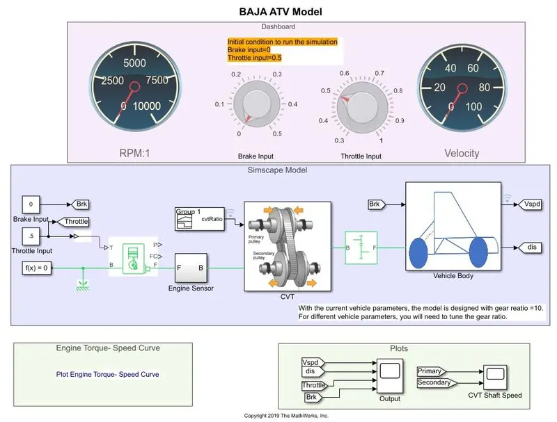
1. Dashboard block which contains

• Engine speed inidcator
• Braket input
• Throttle input
• Vehicle velocity indicator

2. Simscape model block which contains

• Brake input (Transfer from Dashboard block through constant)
• Throttle input (Transfer from Dashboard block through constant)
• Engine
• Engine sensor (To measure speed)
• Simple gear (Gear ratio = 10)
• CVT Ratio (Signal Builder)
• CVT block (To have indefinite gear ratios)
• Vehicle body

3. Plot of Engine torque - speed curve

4. Plots which shows the following data

• Vehicle speed
• Distance travelled
• Throttle demand
• Brake load
• Primary shaft speed
• Secondary shaft speed

Vehicle body block:

Consists of the following

• Double brake shoe
• Front and Rear wheels
• Vehicle block
• Shaft inertia

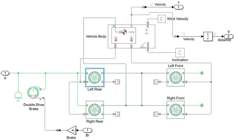
Working of Vehicle body:

• Output from Simple gear train is connected to Rear Wheel (Port 'A'), which in turn develops the thrust (Port 'H') in the Tire (for moving the vehicle) through the Wheel drum.
• Brake input is applied to Rear wheel through the brake shoes (Port 'S' of Brake shoe). Also, shaft inertia is considered for the drive input to the Rear wheels.
• Vehicle body block is given the drive through the thrust (Port 'H') developed by the tire (Port 'H' of Tire block).
• Front and Rear normal wheel forces are applied to the wheels through the Vehicle body block (NF and NR).
• External additional mass is not considered in the Vehicle model.

Vehicle body parameters:

• Mass of Vehicle = 250 kg
• Number of wheels per axle = 2
• Horizontal distance from CG to front axle = 1 m
• Horizontal distance from CG to rear axle = 0.35 m
• CG Height above ground = 0.7 m

Tire parameters

• Rated vertical load = 2060 N
• Peak longitudinal force at rated load = 1260 N
• Slip at peak force at rated load = 5%

• Rolling radius = 0.2921 m
• Tire inertia = 0.01 kg-m^2
• Rolling resistance, constant coefficient = 0.015
• Rolling resistance, velocity threshold = 0.1 m/s
• Rolling resistance is provided to all the wheels.

CVT block:

• CVT block gets the speed input from the Engine and CVT ratio from Signal builder.
• There are 2 shafts in CVT as Primary shaft and secondary shaft.
• Primary shaft speed is same as Engine speed.
• Secondary shaft speed varies based on the CVT ratio as defined in the Signal builder.
• Shaft inertia's are considered during the input and output of the CVT block.

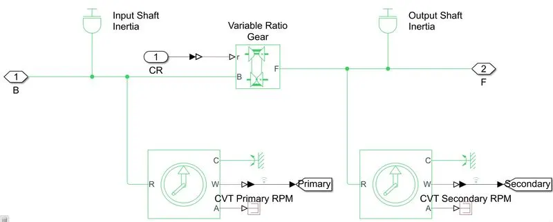
CVT block parameters:

• Input shaft inertia = 0.0154 kg-`m^2`
• Output shaft inertia = 0.0158 kg-`m^2`
• CVT ratio -> Signal builder
• Primary and secondary shaft speed is measured using Ideal rotational motion sensor.

Engine block:

• Input to the Engine block is the throttle demand, which is given as a percentage of the maximum possible torque.
• Throttle input is the torque demanded from the engine.
• Output of the Engine block is the Crankshaft speed which produces the corresponding torque. (i.e the demanded torque).

Engine block parameters:

• Speed = speedVector (stored variable in the Matlab workspace - vector containing 70x1 data), rpm
• Torque = torqueVector (stored variable in the Matlab workspace - vector containing 70x1 data), N-m
• Engine inertia = 0.008 kg-`m^2`
• Initial speed = 1750 rpm
• This block also provides Engine power and Fuel consumption but it is not used in the simulation.

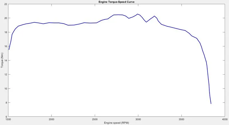
Engine Torque-Speed curve is as shown above.

Simple gear block:

• It is a simple gear block with a fixed gear ratio = 10.

Simulation run observation:

1. Throttle input = 0.5 (Start of Simulation)

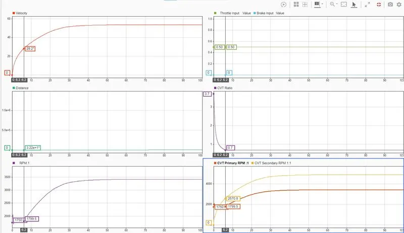
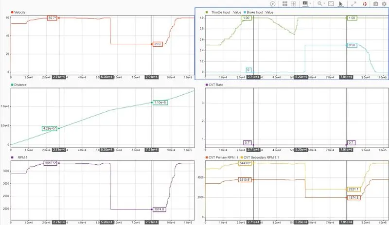
• Simulation is started with the Throttle input as 0.5 and Brake input as 0. At starting speed of Engine is observed to be 1750 rpm. (Refer below figure)
• From 2.9 sec onwards, the CVT secondary shaft rpm starts to increase than the Primary shaft rpm. (This is the point at which the CVT ratio = 1).
• From 1.2 sec to 5.4 sec, Engine speed is 1760~1790 rpm.
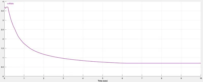
• CVT ratio continues to decrease from 3.7 and after 6.2 sec, CVT ratio remains constant (0.7).

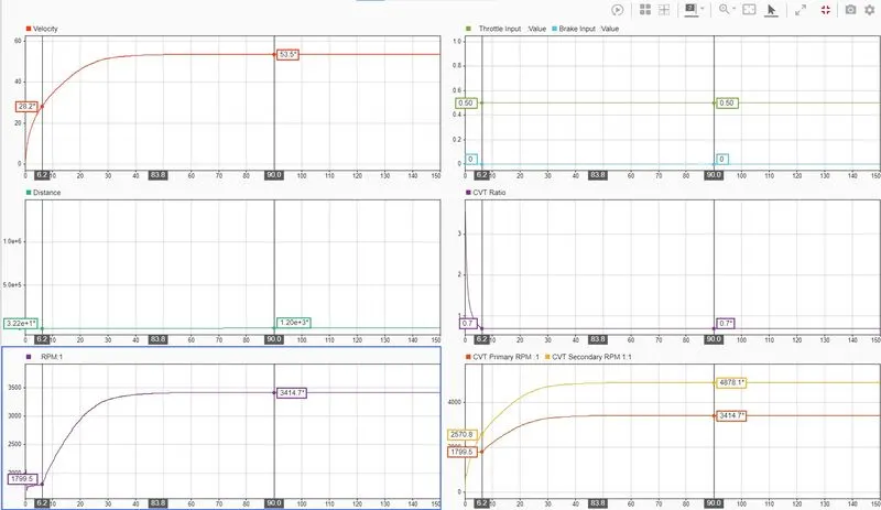
• Once the CVT ratio has reached constant value, Engine speed starts to increase from 1800 rpm and reaches steady value around 3415 rpm.
• This results in the vehicle speed of around 53.5 km/hr.

2. Throttle input is varied from 0.5 to 1 and the observations as follows:

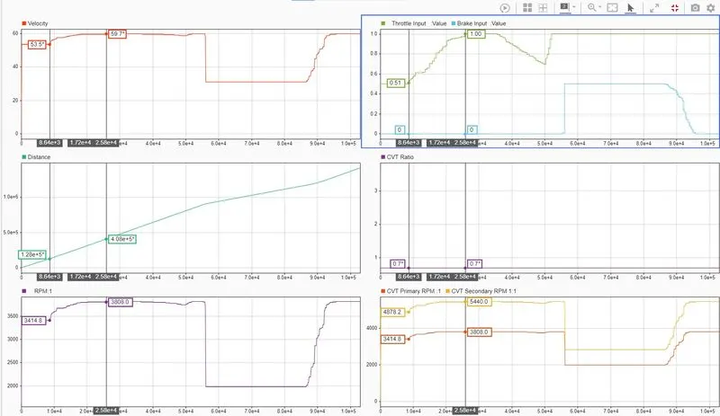
• Engine speed increases from 3414 rpm to 3808 rpm, similarly the secondary shaft speed increases from 4878 rpm to 5440 rpm.
• This results in increased speed of the vehicle from 53.5 km/hr to 59.7 km/hr.

3. Throttle input constant = 1 and Brake input varied from 0 to 0.5

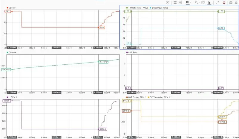
• As the brake input is increased, Engine speed reduces from 3810 to 1975 rpm and subsequently vehicle speed reduces from 59.7 to 31 km/hr.

4. Brake input set back to 0 (Throttle input constant = 1)

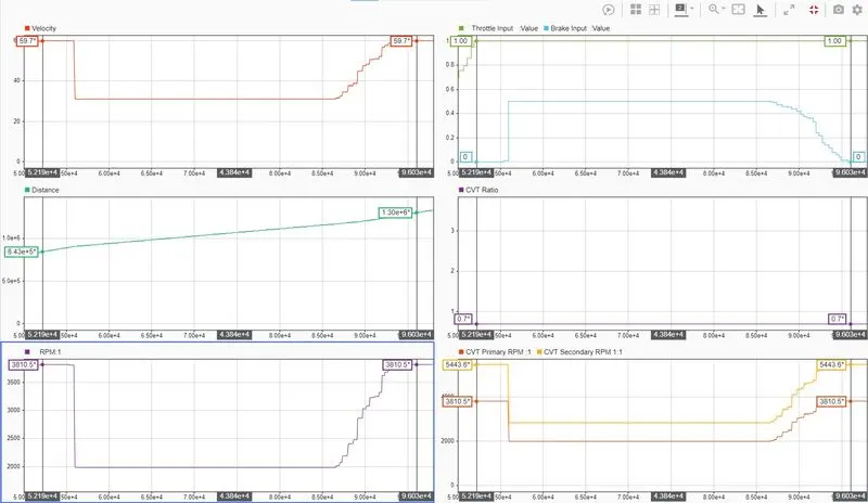
• As the brake input is set 0. Engine picks up the speed back to 3810 rpm and vehcile speed increases to 59.7 km/hr.

Study-2:

The simulink model consists of the following.

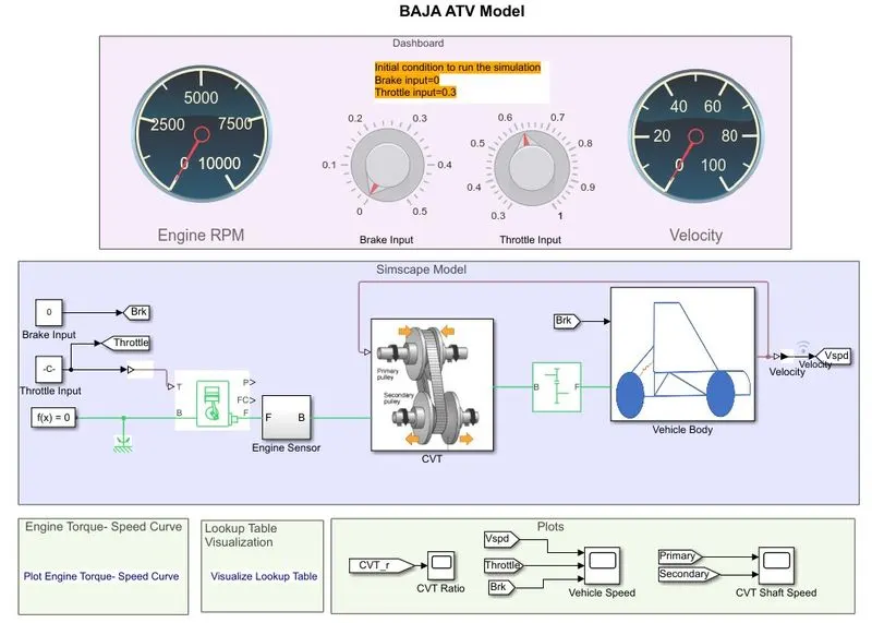
1. Dashboard block which contains

• Engine speed inidcator
• Braket input
• Throttle input
• Vehicle velocity indicator

2. Simscape model block which contains

• Brake input (Transfer from Dashboard block through constant)
• Throttle input (Transfer from Dashboard block through constant)
• Engine
• Engine sensor (To measure speed)
• Simple gear (Gear ratio = 12)
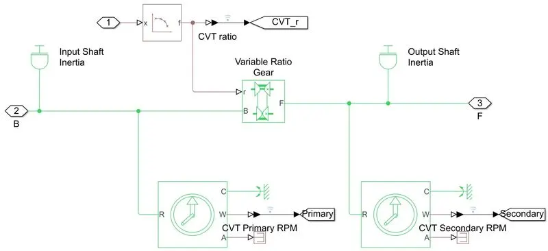
• CVT block (To have indefinite gear ratios) containing CVT Ratio (PS Lookup table (1-D)), for which the input is the output of Vehicle speed from the Vehicle body block.
• Vehicle body

3. Plot of Engine torque - speed curve

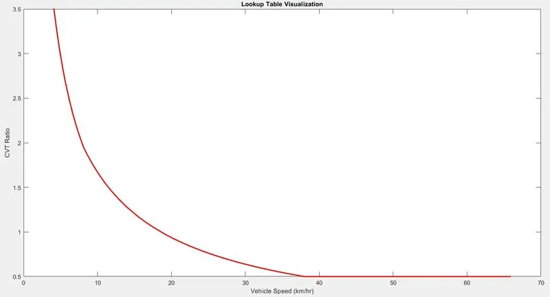
4. Look up table visualization (CVT Ratio vs Vehicle speed plot)

5. Plots which shows the following data

• CVT Ratio
• Vehicle speed
• Throttle demand
• Brake load
• Primary shaft speed
• Secondary shaft speed

Vehicle body block:

Consists of the following

• Double brake shoe
• Front and Rear wheels
• Vehicle block
• Shaft inertia

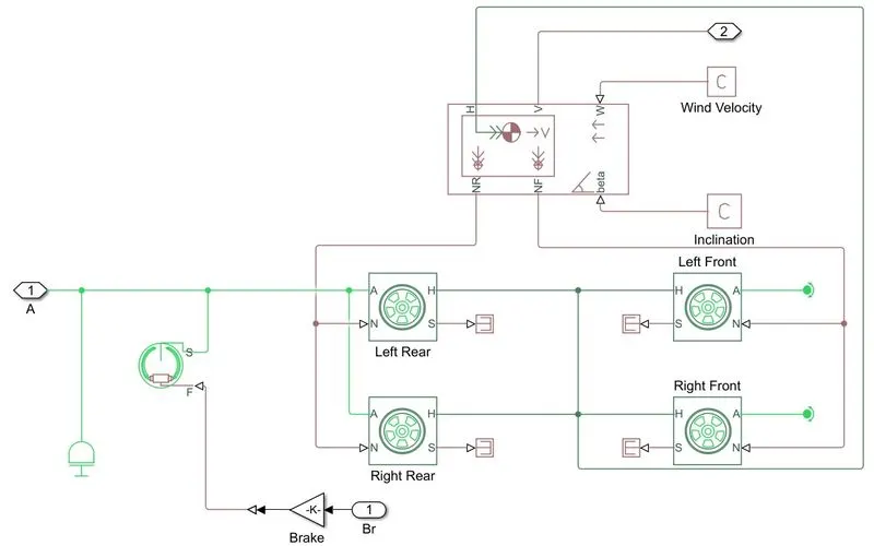
Working of Vehicle body:

• Output from Simple gear train is connected to Rear Wheel (Port 'A'), which in turn develops the thrust (Port 'H') in the Tire (for moving the vehicle) through the Wheel drum.
• Brake input is applied to Rear wheel through the brake shoes (Port 'S' of Brake shoe). Also, shaft inertia (0.1 kg-m^2) is considered for the drive input to the Rear wheels.
• Vehicle body block is given the drive through the thrust (Port 'H') developed by the tire (Port 'H' of Tire block).
• Front and Rear normal wheel forces are applied to the wheels through the Vehicle body block (NF and NR).
• External additional mass is not considered in the Vehicle model.

Vehicle body parameters:

• Mass of Vehicle = 250 kg
• Number of wheels per axle = 2
• Horizontal distance from CG to front axle = 1 m
• Horizontal distance from CG to rear axle = 0.35 m
• CG Height above ground = 0.7 m
• Frontal area = 0.735482 m^2
• Drag coefficient = 1.92
• Air density = 1.18 kg/m^3

Tire parameters

• In this model. instead of specifying the Rated vertical load and longitudinal force, it is Parameterized by "Constant Magic formula coefficients" as follows
• Magic formula B coefficient = 10
• Magic formula C coefficient = 1.9
• Magic formula D coefficient = 1
• Magic formula E coefficient = 0.97

• Rolling radius = 0.2794 m
• Tire inertia = 0.01 kg-m^2
• Rolling resistance, constant coefficient = 0.015
• Rolling resistance, velocity threshold = 0.001 m/s
• Rolling resistance is provided only to Rear left wheel.

CVT block:

• CVT block gets the speed input from the Engine and feedback from Vehicle body block about the Vehicle speed.
• There are 2 shafts in CVT as Primary shaft and secondary shaft.
• Primary shaft speed is same as Engine speed.
• Secondary shaft speed varies based on the CVT ratio as defined in the PS Lookup table (1-D) (Linear interpolation and Extrapolation method is adopted).
• Shaft inertia's are considered during the input and output of the CVT block.

CVT block parameters:

• Input shaft inertia = 0.0154 kg-`m^2`
• Output shaft inertia = 0.0158 kg-`m^2`
• CVT ratio -> PS Lookup table (1-D), X-axis = vehicle_speed/3.6 and Y-axis = cvtr, (where vehicle_speed and cvtr are stored variables in the Matlab workspace - vector containing 252x1 data)
• Primary and secondary shaft speed is measured using Ideal rotational motion sensor.

Engine block:

• Input to the Engine block is the throttle demand, which is given as a percentage of the maximum possible torque.
• Throttle input is the torque demanded from the engine.
• Output of the Engine block is the Crankshaft speed which produces the corresponding torque. (i.e the demanded torque).

Engine block parameters:

• Speed = speedVector (stored variable in the Matlab workspace - vector containing 70x1 data), rpm
• Torque = torqueVector (stored variable in the Matlab workspace - vector containing 70x1 data), N-m
• Engine inertia = 5 kg-`m^2`
• Initial speed = 1600 rpm
• This block also provides Engine power and Fuel consumption but it is not used in the simulation.

Engine Torque-Speed curve is same as Study-1.

Simple gear block:

• It is a simple gear block with a fixed gear ratio = 12.

Simulation run observation:

1.Throttle input = 0.5 (Start of Simulation)

• Simulation is started with the Throttle input as 0.5 and Brake input as 0. At starting speed of Engine is observed to be 1600 rpm. (Refer below figure).
• Speed increases gradually from 1600 to 2195 rpm (till 40 sec). Thereafter, it increases from 42.8 sec, by the time CVT ratio has become 0.5.
• From 32 sec onwards, the CVT secondary shaft rpm starts to increase than the Primary shaft rpm (This is the point at which the CVT ratio = 1).

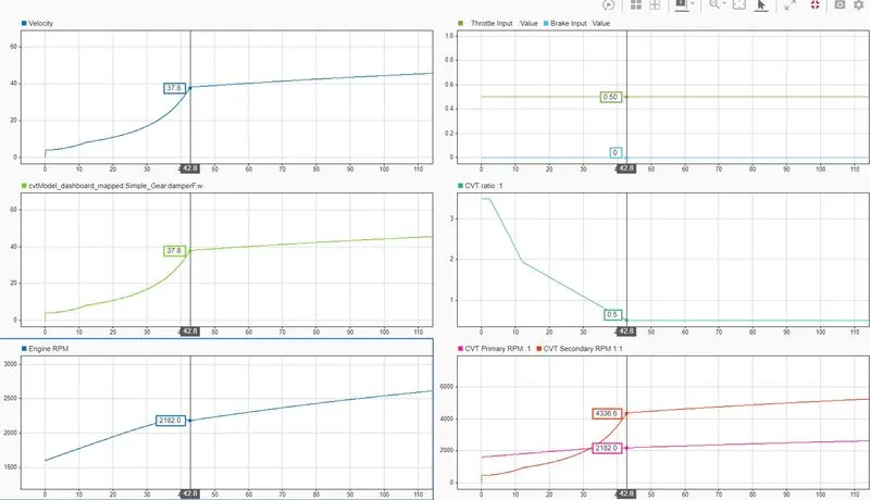
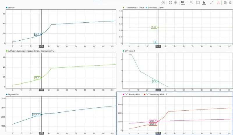
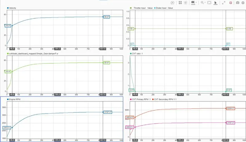
• Once the CVT ratio has reached constant value, Engine speed starts to increase from 2200 rpm and reaches steady value around 3197 rpm.
• Which results in the vehicle speed of around 55.8 km/hr.

2. Throttle input is varied from 0.5 to 1 and the observations as follows:

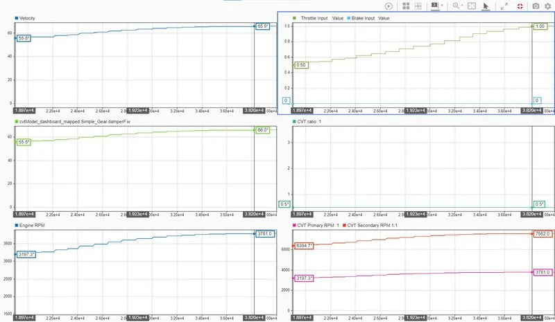
• Engine speed increases from 3197 rpm to 3781 rpm, similarly the secondary shaft speed increases from 6395 rpm to 7562 rpm.
• This results in increased speed of the vehicle from 55.8 km/hr to 66 km/hr.

3. Throttle input constant = 1 and Brake input varied from 0 to 0.5

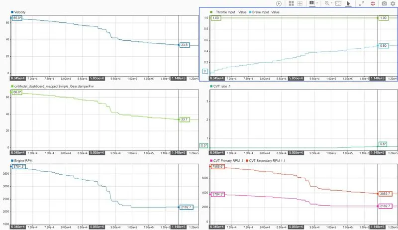
• As the brake input is increased, Engine speed reduces from 3784 to 2182 rpm and subsequently vehicle speed reduces from 66 to 33.7 km/hr.

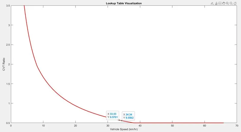
• During this time, as the vehicle speed has come down CVT ratio increases from 0.5 to 0.6.

4. Brake input set back to 0 (Throttle input constant = 1)

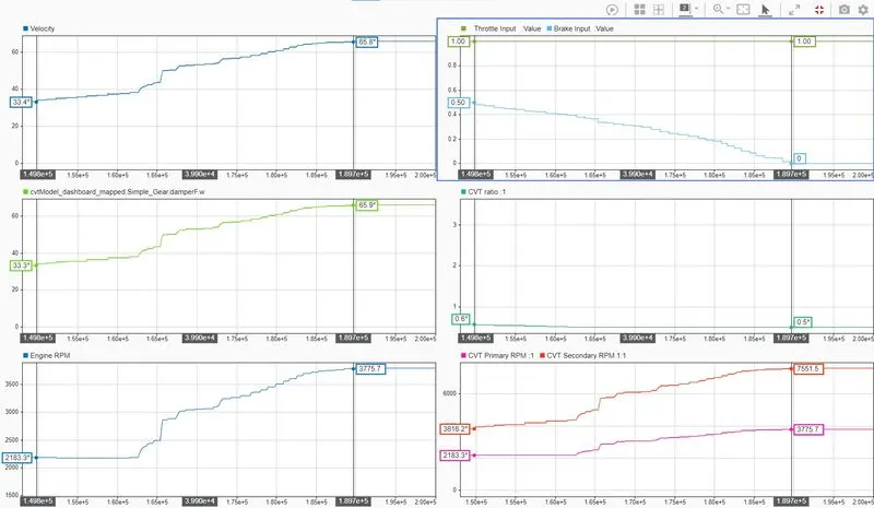
• As the brake input is set 0. Engine picks up the speed back to around 3775 rpm and vehicle speed increases to 66 km/hr.
• Also, the CVT ratio has come back to 0.5 from 0.6.

Conclusion:

STUDy-1 Simulation Plot:

Study-2 Simulation plot:

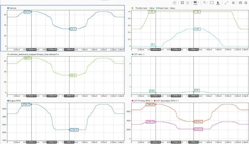
• Compared between the Study-1 and Study-2, CVT ratio is defined as a function of Vehicle speed (in Study-2), which varies the CVT ratio thereby providing improved Torque at lower vehicle speeds.
• Action of CVT is not realized in Study-1, but it is realized in Study-2 (Since it is dependent of Vehicle speed).
• Since, CVT ratio is reduced from 0.7 (Study-1) to 0.5 (Study-2), Vehicle overall speed is higher in Study-2. (Study-1 = 59.7 km/hr and Study-2 = 66 km/hr).
• Overall, Study-2 vehicle model provides improved vehicle performance (Closed-loop feedback).