Project 4

Introduction

The aim of this project is to study the effect of varying Thermal Diffusivities in cases of Pure Diffusion, as well as to compare the effect of applying various Divergence Schemes (for the Convection Term), in cases of Pure Convection using the 3-D Shock Tube tutorial.

Thermal Diffusivity
The Thermal Diffusivity (a material-specific property) is a measure of the rate of heat transfer through the material. In case of a material with high Thermal Diffusivity, heat will move rapidly through it, i.e, it will conduct heat quickly, as compared to it’s Heat Capacity. In essence, it is the measure of Thermal Inertia.

Divergence Schemes
In openFoam, variable values are calculated at the centroids of the cells. However, we also require values at the cell faces. This is achieved by Divergence Schemes, which use the owner’s & neighbour’s centroid data to compute values at the face they share. This arises from the fact that we use the Gauss Divergence Theorem to
convert the Volume Intergral of our Vector Field into a Surface Integral of that Vector over a closed surface, & eventually simplify it as the Summation of Face Fluxes. OpenFoam uses the Rhie-Chow Interpolation to calculate the Face Flux phi.

Case Set-up

I copy the shockTube tutorial from rhoPimpleFoam to my RUN directory. Then, I replace the following files with their counter-parts from cavityTemp (Project-3) :
• controlDict
• fvSchemes
• fvSolution
• transportProperties

All the cases will be run for 5 seconds using the icoTempFOAM solver. Now we must make the following changes to the following files :

2.1 system/setFieldsDict
Here, we wish to specify a region in the middle of the domain where T = 1 Kelvin. Everywhere else, T is specified to be 0 Kelvin. We want to observe how the Temparature Profile varies when subjected
to different conditions. Therefore, we add the following :

defaultFieldValues
(
volVectorFieldValue U (0 0 0 )
volScalarFieldValue T 0. 0
volScalarFieldValue p 100000
) ;

regions
(
boxToCell
{
box (−0.5 −1 −1) ( 0 . 5 1 1 ) ;
fieldValues
(
volScalarFieldValue T 1. 0
) ;
}
) ;

0/p

Here, we must change the dimensionSet for Pressure, as the shockTube tutorial was originally meant to run with a Compressible Solver (rhoPimpleFoam), however, we are going to run it with our custom Incompressible Solver (icoTempFOAM). This is because Incompressible Solvers use the Density Normalized Pressure, rather
than Pressure. Hence, for Compressible Cases, the following dimensionSet is used : [1 -1 -2 0 0 0 0], whereas for Incompressible Cases, the following is used : [0 2 -2 0 0 0 0]. Therefore, we must change
the dimensionSet for Pressure from the former to the latter.

Pure Diffusion

Running the Simulations
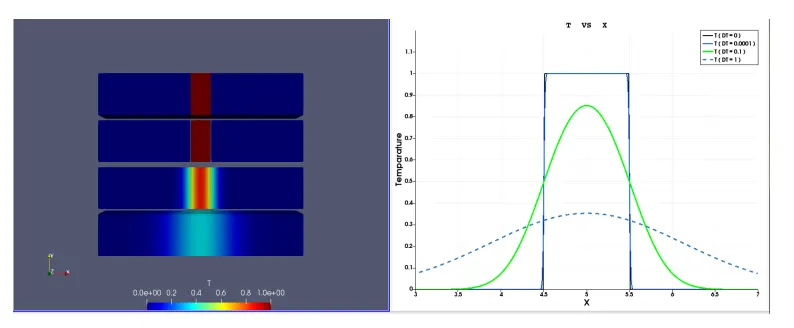
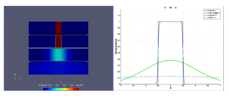
Here, we ignore any sort of Convection effects by setting the value of Velocity to be 0. Now we shall run 4 cases with the following values of the Difussion Coefficient (inside constant/transportProperties), in order:

• DT = 0
• DT = 0.0001
• DT = 0.1
• DT = 1

We execute the following commands for each of these cases to run the simulation :

• blockMesh : This will create the mesh as specified in blockMeshDict.
• setFields : This will set the desired fields.
• icoTempFOAM : This will run the simulation.

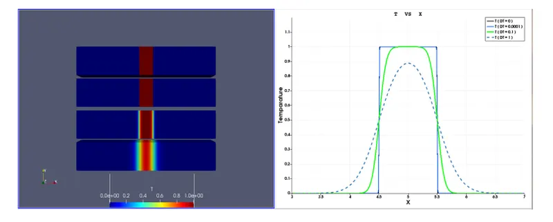
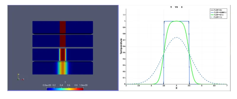
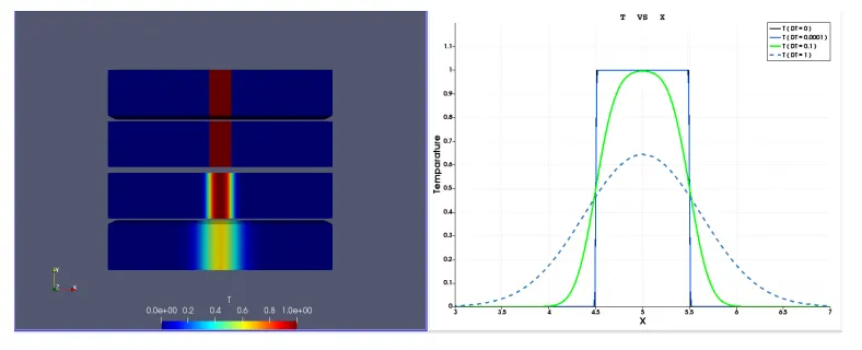
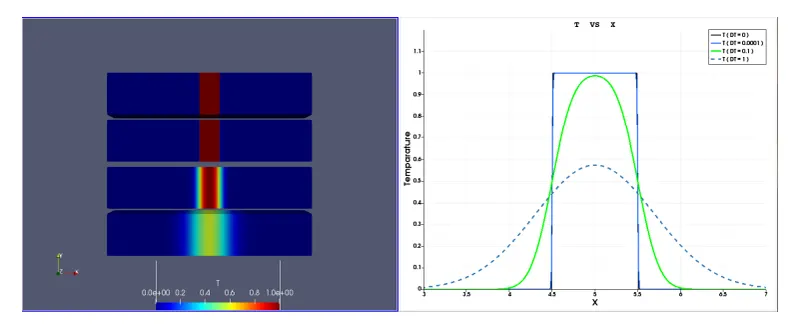
The following will help visualize things better. The animations in the left depict the change in the Temparature field when subjected to different values of the Diffusion Coefficient (in the above order), whereas the graph on the right represents a T vs X plot for all the above cases.

t = 0.05 s

t = 0.1 s

t = 0.15 s

t = 0.2 s

t = 0.6 s

t = 5 s

Interpreting the Results

The simulations give physically realistic results. As is expected, the case with DT = 0 has no diffusion whatsoever (the graph for which is identical for the first & the last time-steps). On the other hand, the case with DT = 1 experiences the maximum amount of diffusion (in the very first time-step, the peak T reduces below the specified T & during the last time-step, it has diffused so much that it can no longer be distinguished). The cases for DT = 0 & DT = 0.0001 give very simillar results, which can only be distinguished by looking at the last time-step. Simillarly, the cases having DT = 0.1 & DT = 1 produce simillar results, but at the same time being more distinguishable as compared to the previous pair.

Pure Convection

Running the Simulations
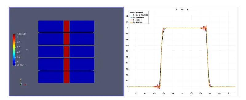
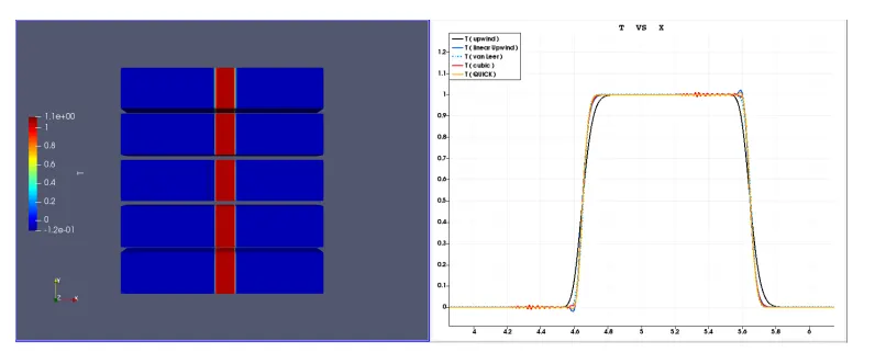
Now, we switch off Diffusion by specifying DT = 0, inside transportProperties & enable Convection by specifying U = 1 m/s inside constant/U. In this section, our objective is to compare & contrast between various Divergence Schemes (applied to div(phi, T)). Now, we shall run 5 different cases with the following Divergence Schemes (by modifying system/fvSchemes), in order :

• Gauss upwind
• Gauss linearUpwind
• Gauss cubic
• Gauss QUICK
• Gauss vanLeer

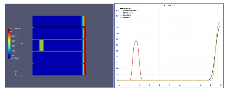
We then run the same 3 commands as before, i.e, blockMesh, setFields & icoTempFOAM. The following will help visualize things better. The animations in the left depict the change in the Temparature field upon varying the Divergence Scheme for Temparature (in the above order), whereas the graph on the right represents a T
vs X plot for all the above cases.

t = 0.05 s

t = 0.15 s

t = 1.55 s

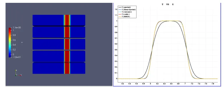
t = 2.25 s

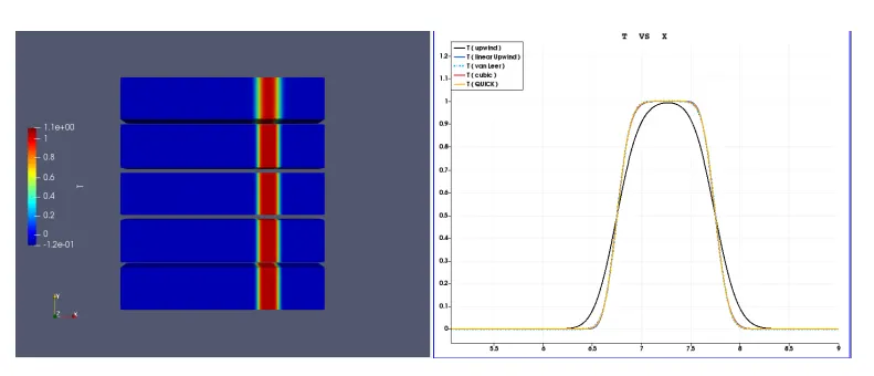
t = 3.3 s

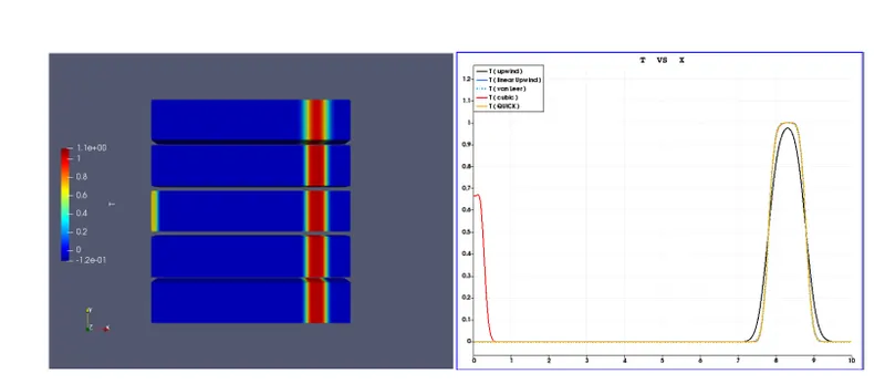
t = 4.25 s

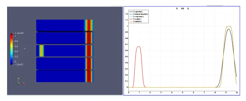
t = 5 s

Interpreting the Results
These sets of simulations do not give physically realistic results. Infact, they expose a serious flaw in Lower Order Divergence Schemes, which is False Diffusion. As is evident, even though diffusion is switched off, all of the above cases depict some degree of diffusion. This is known as Numerical Diffusion or False Diffusion, which occurs primarily due to the Truncation Errors in Lower Order Schemes. It may be noted that, this error still exists in TVD Schemes (such as Van Leer), but is less in magnitude when compared to Lower Order Schemes (such as Linear Upwind). It is extremely interesting to note the Ghost Oscillations while using the Cubic Scheme, which is evident from the data of the last time-steps, where we can see an additional Temparature region that is completely phisically unrealistic. Furthermore, all of the above schemes (except Van Leer) result in Parasitic Oscillations near regions of sharp gradients or discontinuities, which is the preimary reason for the need of TVD (Total Variation Diminishing) Schemes. To conclude, among all the
above, the Van Leer Divergence Scheme produces the best results.

Conclusion
This project sheds light into the phenomena of Convection & Diffusion, as implemented in openFoam. Since we treated these two separately, it revealed a significant flaw in Lower Order Divergence Schemes, i.e, Numerical/False Diffusion, which would otherwise have been masked by Actual/Real Diffusion. In reality, however, both these phenomena occur simultaneously, thereby mandating the use of TVD Schemes, which give the most satisfactory results.