Project
SIMULATION OF AN ALL TERRIAN VEHICLE - System Level.
AIM:
Carry out a system-level simulation of an all-terrain vehicle and to Prepare a technical report explaining the model properties.
INTRODUCTION:
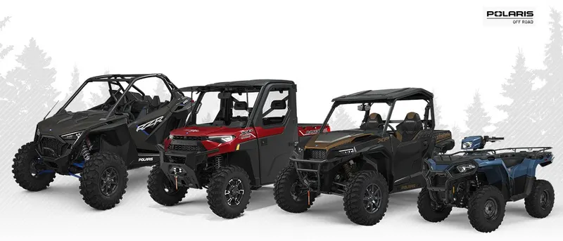
- An all-terrain vehicle (ATV), also known as a light utility vehicle(LUV), a quad bike, or simply a quad.
- It is a vehicle that travels on low-pressure tires, with a seat that is straddled by the operator, along with handlebars for steering control.
- As the name implies, it is designed to handle a wider variety of terrain than most other vehicles.
- By the current ANSI definition, ATVs are intended for use by a single operator, although some companies have developed ATVs intended for use by the operator and one passenger.
- These ATVs are referred to as tandem ATVs.
SIMULATION:
- The model taken for the Simulation is the BAJA ATV model with Continously Variable Transmission (CVT).
- We are going to preapare a study with the following studies:
- BAJA ATV model without dashboard
- BAJA ATV model with dashboard
- BAJA ATV model using the lookup table without a dashboard
- BAJA ATV model using the lookup table with a dashboard.
TOOLS: Matlab, Simulink.
BAJA ALL TERRIAN VEHICLE:
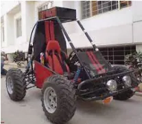
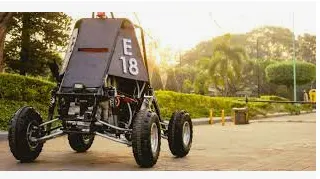
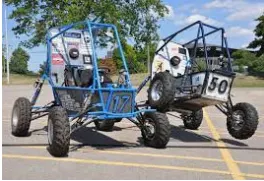
- BAJA is basically an ATV competition where students get to design and develop their own ATV keeping in mind various considerations of design as well as safety.
- An ATV is designed in order to run on various terrains such as soil, Gravel, pebbles, etc.
CONTINUOUSLY VARIABLE TRANSMISSION (CVT):
- the job of the transmission is to change the speed ratio betwen the engine and the wheels of an automobile.
- the transmision uses a range of gears-from low to high to make more effecitive use of the engine's torque as driving conditions change.
- the gears can be engaged manually or automatically.
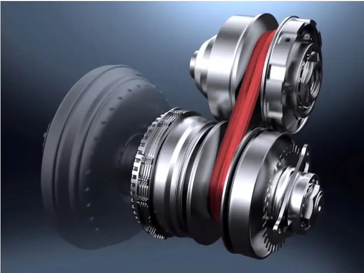
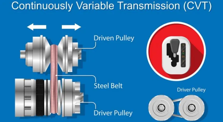
- a continous variable transmission -CVT is a transmission that can change seamlessly through an infinte number of effective gear
ratios between maximum and minimum values. - IN a CVT transmission, the pushbelt transfers the torque from one pulley to the other.
- The level of power transmission is adapted automatically through continuous varibale adjustement of the pulleys.
ADVANTAGES OF CVTs:
- Allows for an infinite number of gear ratios.
- Eliminates "Shift shock" - makes it smoother ride.
- Responds better to changing conditions.
- Better fuel economy and reduced power loss.
CASE 1: BAJA ATV MODEL WITHOUT DASHBOARD:
for our case 1 study we are going to Simulate the BAJA ATV MODEL without Dashboard.
SIMULINK MODEL:
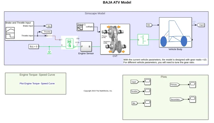
- the BAJA ATV model consists of Signal builder which provides the brake and throttle input as a signal.
- The signal builder block is connected to a generic engine block where the block's rotational ports are connected with
a Rotational reference and a solver configuration to provide simulation. - the engine is connecte to the engine sensor and the engine sensor is connected to the CVT gear box which has a
connected with a CVT ratio signals. - the CVT Block is connected with a simple gear boc and then connected to the Vehicle body.
- all the block are tagged and connected to the scopes.
- lets discuss more in details.
MODEL EXPLANATION:
- The purpose of creating this model is to examine the behaviour of the vehicle in response to the brake and throttle input.
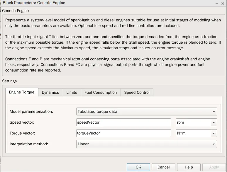
- The brake and throttle inputs are fed to the generic engine using a signal builder block. In the generic engine block, the speed and torque values are defined in the script file.
- The o/p from the generic block is fed to the engine sensor subsystem.
- CVT ratio block is used to vary the CVT ratio.
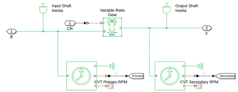
- The engine senor o/p and the CVT ratio block o/p is fed to CVT. In the CVT subsystem, the i/p at the primary shaft is fed to variable gear ratio whose varied o/p is measured at the output shaft.
- Rotational motion sensors are connected to both the shafts to measure the speed. The output of CVT is fed to vehicle body subsystem where it is transferred to wheels connected to the axles.
- When the throttle is at its maximum, maximum velocity is obtained in the ATV. According to the brake input applied, the vehicle comes to stop. In this model no brakes are applied.
SIGNAL BUILDER - BRAKE AND THROTTLE INPUT:
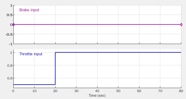
- The brake input remains 0 throughout 80 secs.
- The throttle input remains at 0.5 for first 20 secs and then increases to 1 and remains the same throughout the 80 secs.
GENERIC ENGINE:
- The Generic Engine block represents a general internal combustion engine.
- Engine types include spark-ignition and diesel.
- Speed-power and speed-torque parameterizations are provided.
- A throttle physical signal input specifies the normalized engine torque.
- Optional dynamic parameters include crankshaft inertia and response time lag.
- A physical signal port outputs engine fuel consumption rate based on choice of fuel consumption model.
- Connections F and B are mechanical conserving ports associated with engine crankshaft and engine block.
- Ports P and FC are physical signal ports.
- The speed and torque vector values are obtained from the graph and can be viewed form the Matlab workspace.
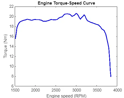
- As observed from the graph, the torque value is high and it increases until the engine attains its maximum speed and then starts to fall.
- In this model, the max. engine speed is 3840 rpm.
Engine sensor:
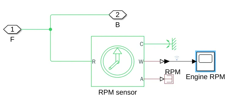
- The Ideal Rotational Motion Sensor (RPM sensor) block represents an ideal mechanical rotational motion sensor, that is, a device that converts an across variable measured between two mechanical rotational nodes into a control signal proportional to angular velocity or angle.
- Connections R and C are mechanical rotational conserving ports that connect the block to the nodes whose motion is being monitored.
- Connections W and A are physical signal output ports for velocity and angular displacement, respectively.
- The block positive direction is from port R to port C.
Signal builder (CVT ratio):
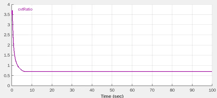
The CVT gear ratio initiates from 3.8 and gradually falls to 0.8 and thereafter it remains constant till 100.
CVT Subsystem:
- Inertia:By default, the block has one mechanical translational conserving port. The block positive direction is from its port to the reference point. This means that the inertia torque is positive if inertia is accelerated in positive direction.
- Variable Ratio Transmission block: This represents a gearbox that dynamically transfers motion and torque between the two connected driveshaft axes, base and follower. Ignoring the dynamics of transmission compliance, the driveshafts are constrained to corotate with a variable gear ratio that you control. You can choose whether the follower axis rotates in the same or opposite direction as the base axis. If they rotate in the same direction, ωF and ωB have the same sign. If they rotate in opposite directions, ωF and ωB have opposite signs.
Simple gear:
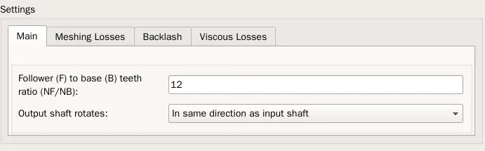
- The Simple Gear block represents a gearbox that constrains the connected driveline axes of the base gear, B, and the follower gear, F, to corotate with a fixed ratio that you specify.
- You choose whether the follower axis rotates in the same or opposite direction as the base axis.
- If they rotate in the same direction, the angular velocity of the follower, ωF, and the angular velocity of the base, ωB, have the same sign.
- If they rotate in opposite directions, ωF and ωB have opposite signs.
- The NF/NB ratio is given as 12 and the o/p shaft rotates in the same direction as i/p shaft.
Vehicle body subsystem:
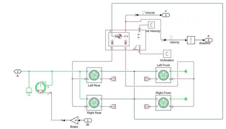
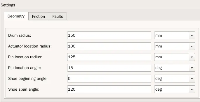
- Double shoe brake: The Double-Shoe Brake block represents a frictional brake with two pivoted rigid shoes that press against a rotating drum to produce a braking action. The rigid shoes sit inside or outside the rotating drum in a diametrically opposed configuration. A positive actuating force causes the rigid shoes to press against the rotating drum. Viscous and contact friction between the drum and the rigid shoe surfaces cause the rotating drum to decelerate. The following specificationsare fed to the brake.
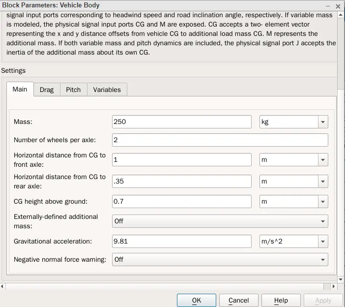
- Vehicle body: The Vehicle Body block represents a two-axle vehicle body in longitudinal motion. The vehicle can have the same or a different number of wheels on each axle. For example, two wheels on the front axle and one wheel on the rear axle. The vehicle wheels are assumed identical in size. The vehicle can also have a center of gravity (CG) that is at or below the plane of travel.
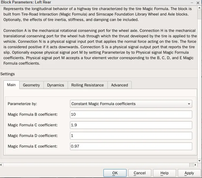
- Tire: The Tire (Magic Formula) block models a tire with longitudinal behaviour given by the Magic Formula. The block can model tire dynamics under constant or variable pavement conditions.The longitudinal direction of the tire is the same as its direction of motion as it rolls on pavement. This block is a structural component based on the Tire-Road Interaction (Magic Formula) block. The parameters for the tire are being fed and this applies for all the other 3 tires.
OUTPUT:
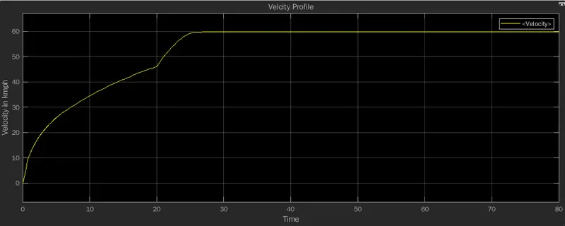
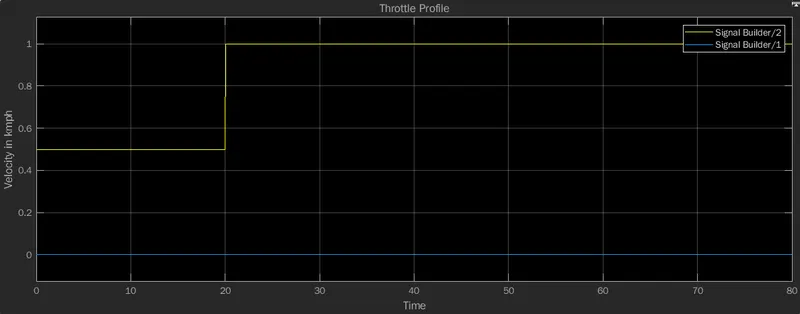
- From the graph we can see that the velocity is 0 when the throttle input is 0.5.
- The velocity steadily increases for 20 secs and at 20 secs the velocity value is 45.
- Now at 45 secs, the throttle input is given fully and the velocity value increases and reaches a maximum value and continues to remain constant thereafter.
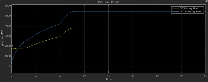
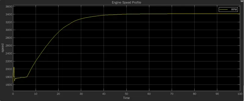
- from the speed profile graph we can understand that the Secondary rpm is higher than the primary CVT RPM.
- the speed at primary starts ar 1800 rpm and jumps to 2000 and comes back to 1800 creating a spike and gradually increases and maintains the constant speed
with respect to the time. - where in the secondary CVT RPM graph it starts at 0 and gradually inceares after 30 seconds it maintains a constant speed
with respect to the time.
CASE 2: BAJA ATV MODEL WITHOUT DASHBOARD:
A Simulink model of the BAJA ATV model with dashboard is shown below. All the other systems are the same as the previous Simulink model.
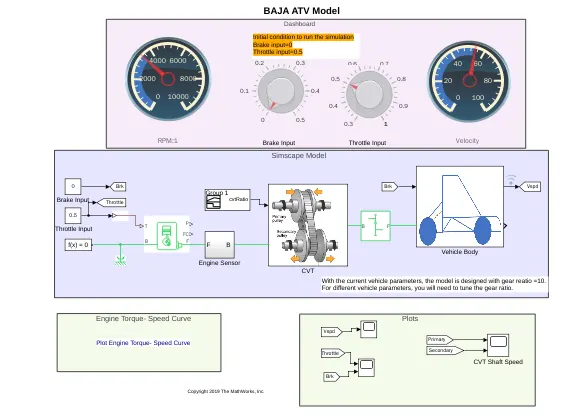
- The only difference here compared with the previous model is that, a variable brake and throttle input is given.
- The input is varied using a knob. The output for the varied throttle and speed is viewed from the rpm and velocity gauge.
- The initial conditions of the brake is 0 and throttle is 0.5.
OUTPUT:
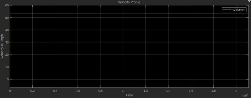
it can be observed form the graph that the velocity increases drastically form 0 to 53 kmph when the throttle value is 0.5 and brake input is 0.
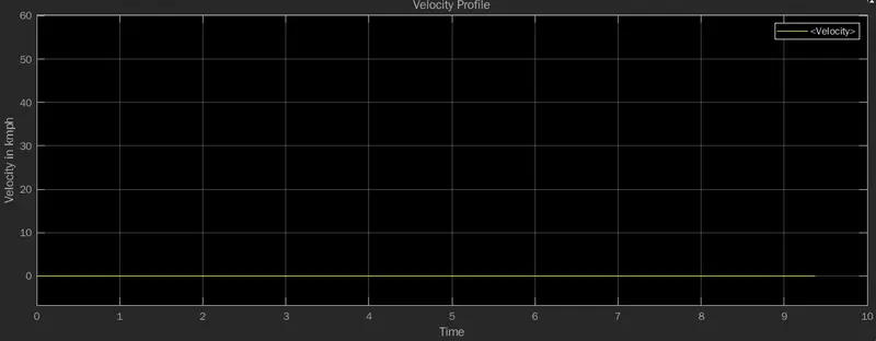
lets, change the brake input from 0 to 1,we can observe that when braking is applied the moment of the baja is arrested and the value in the graph carries 0 throughout.
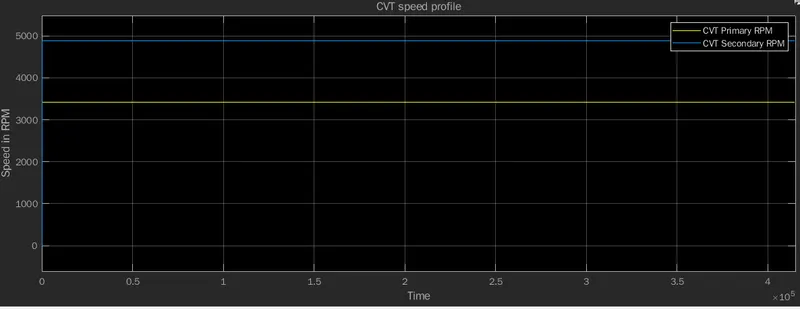
- this graph shows us the characteristics of speed from the CVT gear box.
- We can observe that both the Primary CVT and Secondary CVT are same till 3300 rpm.
- then we can see that secondary CVT RPM is higher than the Primary CVT RPM.
CASE 3: BAJA ATV MODEL WITH LOOKUP TABLE:
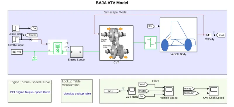
- In this model, the signal builder inputs are replaced as two step blocks one for each input.
- Also the CVT ratio signal builder block is removed.
- Instead the output velocity is fed back to the CVT block.
- The CVT block adjusts the CVT ratio in accordance with the lookup table.
- All the other systems are the same as discussed in the above two methods.
LOOKUP TABLE:
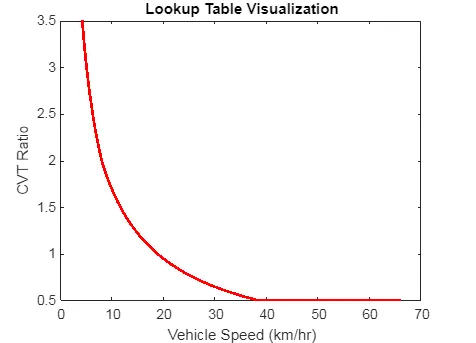
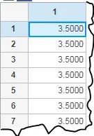
- A lookup table is an array of data that maps input values to output values, thereby approximating a mathematical function.
- Given a set of input values, a lookup operation retrieves the corresponding output values from the table.
- If the lookup table does not explicitly define the input values, Simulink® can estimate an output value using interpolation, extrapolation, or rounding,
- where:
- An interpolation is a process for estimating values that lie between known data points.
- An extrapolation is a process for estimating values that lie beyond the range of known data points.
- A rounding is a process for approximating a value by altering its digits according to a known rule.
CVT MODEL:
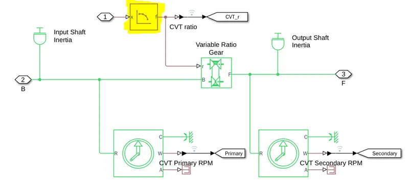
- the only difference between this model and the first model is that in this model the gear ration input to CVT is provided using a lookup table.
- the velocity and shaft rpm outputs are same as before.
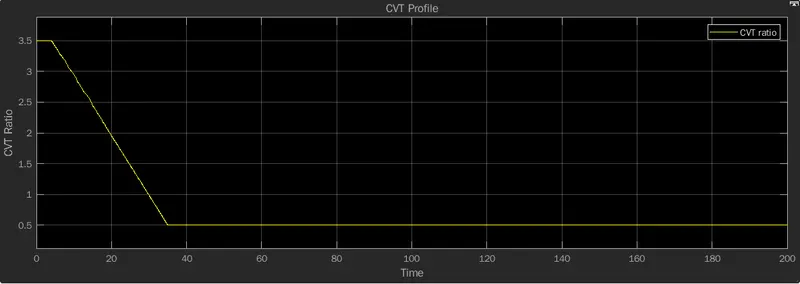
- basically CVT ratio defines that the ratio of Primary speed to the secondary speed with respect to the time.
- in this graph we can observe that the CVT ratio starts form 3.5 and continuous for 4 seconds and then reduces to 0.5 at 38 seconds and maintains the ratio throughout the simulation.
OUTPUT:
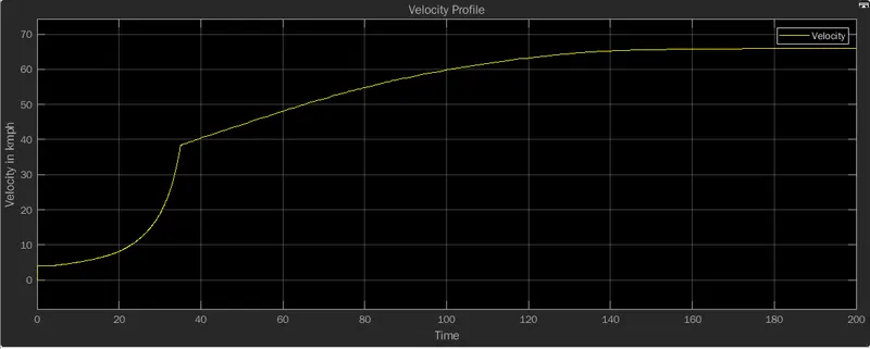
- from the Velocity profile graph we can understand that the velocity increases drastically from 0 to 3 kmph and then reaches 38 kmph in 37 seconds
when the throttle is in 0.3. - when throttle increases from 0 to 1 the veloctity gradually increases from 38 kmph to 65 kmph with respect to time and sustains the level.
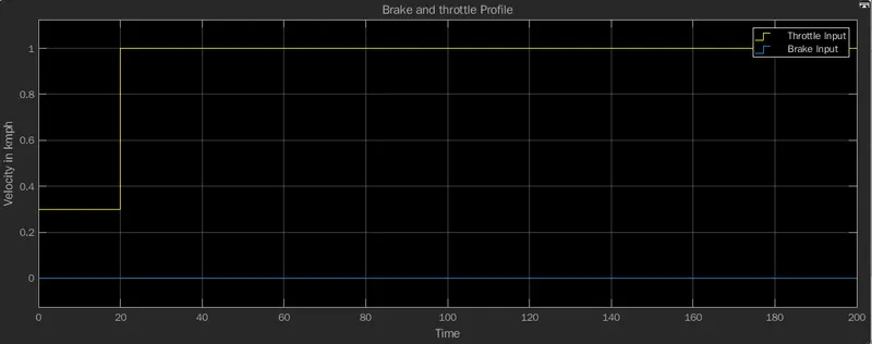
- from this graph we can understand see that the throttle was initially 0.3 and maintians the same velocity for 20 seconds and increases to 1 kmph in 20 seconds and sustains the level. likewise the brake is 0 throughout the simulation.
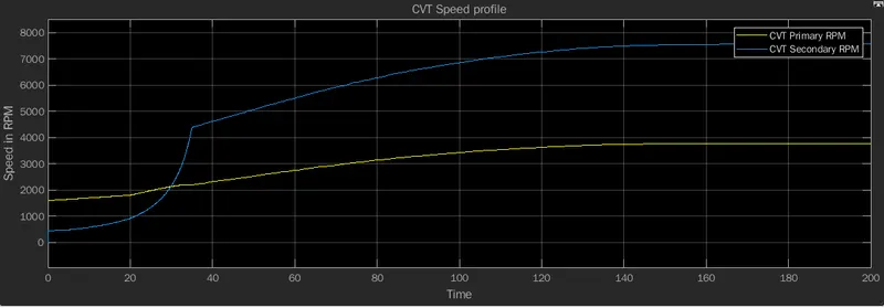
- these graphs shows the variation in angular velocities of input and output shafts of the variable gear transmission system.
- these values differ with respect to the gear ratio. as we can see that the primary rpm starts at 1800 rpm and maintains the speed.
- we can also see that the secondary rpm starts at 0 and increases to 500 rpm in 0 sec and when throttle is 0.3 it gradually increases the speed form 0 to 4300 rpm and when the throttle increases to 0.5 the speed increase to 7500 rpm with respect to time.
CASE 3: BAJA ATV MODEL WITH LOOKUP TABLE AND DASHBOARD:
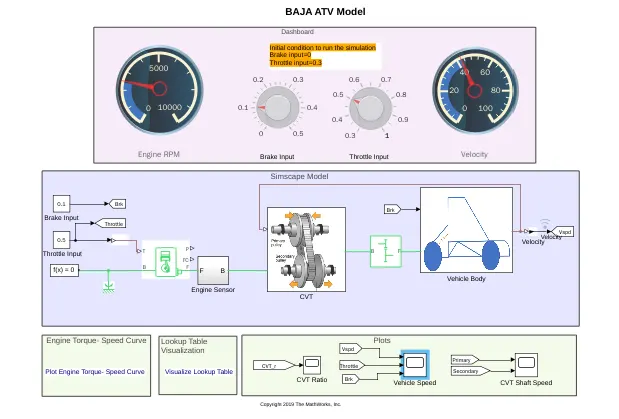
- The only difference here compared with the previous model is that, in this case a variable brake and throttle input is given.
- The input is varied using a knob. The output for the varied throttle and speed is viewed from the rpm and velocity gauge.
- The initial conditions of the brake is 0 and throttle is 0.5.
OUTPUT:
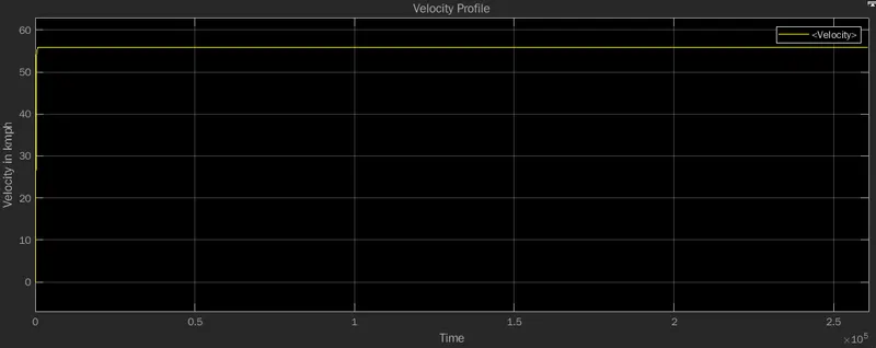
- it can be observed form the graph that the velocity increases drastically form 0 to 55 kmph when the throttle value is 0.5 and brake input in 0.
- the Baja continuous to maintain the 55kmph speed throughout the simulation.
- this graph shows us the characteristics of speed from the CVT gear box.
- We can observe that both the Primary CVT and Secondary CVT are same till 3300 rpm.
- then we can see that secondary CVT RPM is higher than the Primary CVT RPM.
ALL TERRIAN ELECTRIC VEHICLE:
- the electrification of power train allows for an increase in the overal drive train efficiency.
- electrical systems are much more efficient thatn INternal combustion engines.
- They can be used both on road and on uneven terrains which makes them versatile.
- They provide 100% ecofriendly and Noise polution free system.
- Extremely robust and with high performances
- they can be used in Multifunctional areas from a Golf cart to Deserts.
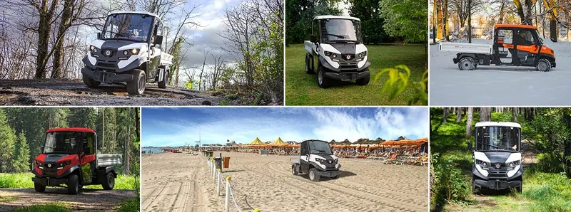
- they can handle the most difficult terrains, that usually require 4×4 vehicle performances.
- Although they have two-wheel drive motors, they have the same performances that characterize off-road 4x4 four-wheel drive vehicles of the same category.
- These vehicles are able to work any ground type and they can work without problems with slippery or uneven terrains, with sand, grass, challenging slopes, snow or ice,
- also thanks to special accessories as the snow blade and the salt spreader.
RESULT:
thus the System level modelling of a All terrain vehicle is sucessfully completed and the technical report expalining the model properties were also completed and the output is verified.