Project
Q.Carry out a system-level simulation of an all-terrain vehicle.
Prepare a technical report explaining the model properties & comments on the results.
A.
Aim:To study and analyze BAJA ATV
OBJECTIVE:Prepare a technical report explaining the model properties & comments on the results.
Facts and History About ATV
|
||
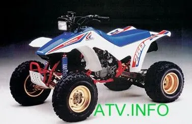
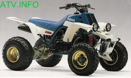
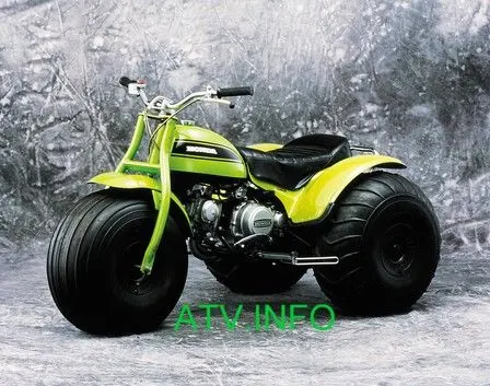 Photo: Honda 1970 ATC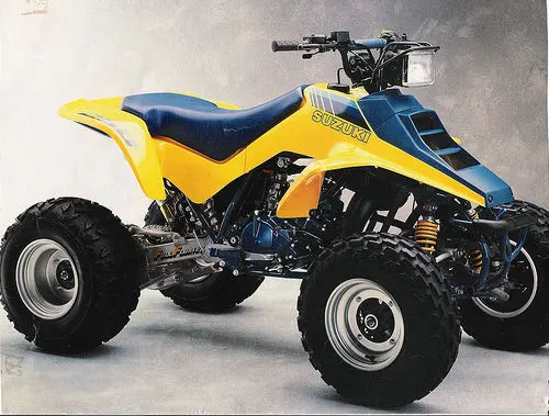
INFORMATION COLLECTED ABOUT ATV FROM IEEE TO CONSTRUCT IT IN REAL TIME.
Using a CAN Bus for Control of an All-Terrain
Vehicle
Abstract—When designing an autonomous All-terrain Vehicle(ATV) one must ensure that the communications paths to all
major subsystems use a robust electrical signaling protocol. Onesuch protocol is the CAN bus. This project describes an effort to utilize a CAN bus to connect existing and new hardware on an ATV. The work involved a redesign of the braking control systemas well as the throttle controls. The redesign was necessary toreplace obsolete or broken components, reduce the amount of extra wiring on board the ATV, and create a robust infrastructurefor future expansion. A CAN bus control node was installed foreach major component on the ATV as well as a master controlnode. The master control node now reads in signals from a remotecontrol receiver and interprets them into commands for the other nodes on the CAN bus. Each node takes the commands received from the CAN bus and drives their respective components. Acontrol node was developed to control the throttle and brakingsystem. A second node was developed to control the steering control system. New control systems were developed for drivingthe brakes and the steering. The ATV can now be driven using aRC controller to operate the brakes, steering, and throttle, and is poised to accept new hardware to make it truly autonomous.
Index Terms—CAN Bus, ATV, Remote Control, RX63N, GRSakura
I. INTRODUCTION
The end goal of this work is to create a fully autonomous ATV. Before making the ATV autonomous, a remote control system needed to be developed. The ATV originally worked by remote control, but many of the original components had been salvaged for other projects. The original microcontroller had to be replaced and all of the wiring had to be redesigned.
A CAN bus was also installed to reduce the amount of wiring
on board the ATV. The CAN bus also makes for easier addition and removal of new components to the system. The steering system had also been redesigned and needed to be integrated
into the new control system. The initial wiring is shown in Figure 2. The control system was broken down into multiple
sections on the CAN bus to make the system more modular.
Each component was assigned to one of three microcontrollers which interpret commands to and from the CAN bus. The control system was seperated into a master control node, a
steering control node, as well as a steering and throttle control node. CAN bus is mostly used in the automotive industry and was developed specifically with cars in mind. CAN bus was
designed to reduce the amount of cable running between all of the sensors and controls inside of a vehicle. Autonomous vehicles typically require a large number of sensors for navigation,
which makes CAN well suited to this application.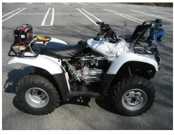
Fig. 1. Zapatabot ATV [5]
II. CAN BUS
A. CAN Bus
Since one of the future goals of this work is to add sensors to make the ATV fully autonomous, a Control Area Network (CAN) bus was chosen[4]. A CAN bus allows for the easy addition and removal of components to the system without disturbing the rest of the bus. A CAN bus requires only twowires and a ground for communication between all nodes on the bus. This greatly reduces the amount of cabling runningthroughout the ATV. When a new node needs to be added to the bus, it simply needs to be connected to the two wires already running throughout the ATV. This simplifies addition and removal of nodes over the initial setup. A master control node was developed which interprets the RC controller signals into CAN messages and then transmits them to the other nodes. Another node was also made for controlling the brakes and the throttle. This node reads messages from the CAN bus and interprets them into directions for the brakes and throttle. The steering control node works the same way by interpreting CAN messages into commands to the steering system. A diagram of the overall plan for the CAN bus is 978-1-4799-6585-4/14/$31.00 ©2014 IEEE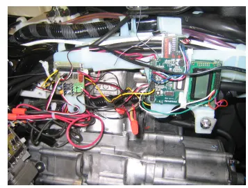
Fig. 2. Initial ATV Wiring [5]
shown in Figure 5.
CAN is an asynchronous TDM protocol. It has a relativelyslow data rate, but makes up for it with very high reliabilit.CAN messages can be heard by all nodes on the bus. Thisallows for easy debugging of multiple components and reducesthe amount of wiring needed to connect each of the nodes for communication. CAN operates using a three wire system.The wires are CAN High, CAN Low, and Ground. Typically CAN devices operate at 5V, but 3.3V devices are also used.In order to communicate via CAN, a CAN module and a CAN transceiver are required. The CAN module is typically embedded into the microcontroller, while the transceiver is an external component. The CAN module is in charge of reading and sending signals to the transceiver and placing valid messages into their respective mailboxes. The CAN transceiveris responsible for converting bits received into a signal across the CAN High and CAN Low wires.
When a 1 is being sent across the bus, both lines are set to 2.5V. When a 0 is sent across the bus, the CAN High line goesto 3.5V and the CAN Low line goes to 1.5V. The transceivers on the bus then use the voltage difference across the lineto determine whether a 1 or 0 is being sent. This is shown in Figure 3.
CAN is unique in the way that it handles bus
arbitration. When two nodes attempt to transmit at the sametime, zeros will overwrite ones. When a node sees that oneof its bits has been overwritten by another node, it will backoff andwait until the message is finished to begin transmitting
again. Since the ID of a message is broadcast first, the first fewbits are often used to indicate the priority of the message. Since
zeros overwrite ones, the ID with the lowest value always has a higher priority. An example is shown in Figure 4.
The SAE J1939 Standard was used in setting up the steeringcontrol node. Since the SAE J1939 standard is common andwas already implemented in the steering node, this protocol
was used for the rest of the system as well. The SAE J1939standard runs at 250kbps. The node for the steering system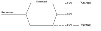 .
.
Fig. 3. CAN Transmission[1]
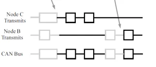
Fig. 4. CAN Arbitration[1]
was developed using a PIC Microchip microcontroller[6]. The steering control node interprets the first two data bytes into a
steering angle for the wheels and then tricks the steering assist into turning the desired direction. In current network the extended ID mode is used which uses
29 bit identifiers instead of the standard 11 bits. In CAN, each message is given an ID. This ID used to indicate the message type instead of the destination. Each device will have multiple
mailboxes with different IDs in order to read in multiple types of messages. Mailboxes are also given a mask so that they can ignore certain bits such as the priority bits. This also means a mailbox could be set up to ignore all of the bits in an ID and receive all messages sent on the bus. In the current network,
the first 3 bits are used to indicate priority. The last 8 bits are used to indicate the source address of the message. The source address mostly goes unused for now, but is useful for debugging and error messages. The rest of the bits are used for the ID and are the only bits not masked out. Each type of message will have its own unique idea. For now, the only
types of commands used are steering, acceleration, braking, and error messages.
A Renesas RX63N microcontroller was used as the master node for giving the rest of the system commands. The master node is also responsible for interpreting signals from the
remote control. The RX63N development board was chosen because it already has both a CAN module as well as a CAN transceiver on board. The board also has CAN APIs available, which simplified programming of the CAN bus. The master node is responsible for most of the messages on the CAN bus. The other two nodes only transmit startup complete and
978-1-4799-6585-4/14/$31.00 ©2014 IEEE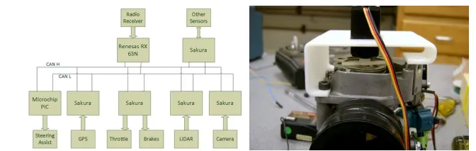
Fig. 5. CAN Design Plan,Fig. 6. Throttle Servo Mount[5]
error messages. This will change in the future, after sensors are added to the ATV.The largest disadvantage to using a CAN bus is that eachcomponent now needs an individual microcontroller to control it. The microcontroller is mainly used to interpret the CANmessages into control signals for the devices it is responsible for. The steering and throttle were originally going to be treated as two seperate nodes. They were combined into one node since neither device has complex controls and neither device will be removed from the system since throttle and braking are required for the ATV to drive. The brakes and throttle are both controlled by a Renesas GR-Sakura microcontroller. Since the Sakura board uses an RX63N microcontroller,it already has a CAN module built in. For the transceiver, a Texas Instruments SN65HVD251 Industrial CAN Transceiver was used. Even though the Sakura uses an RX63N, the CANAPIs could not be used, because the APIs were designed specifically with the RX63N development board in mind.
III. OTHER COMPONENTS
A. Throttle and Brakes
As stated previously, both the throttle and the brakes were controlled using a Sakura microcontroller. The throttle control on the Honda ATV was developed by a previous group
and worked well so no modifications were made other than switching control to the Sakura[?]. The throttle is controlled by a standard Parallax servo attached to the throttle via a rapid
prototyped frame. Since the ATV has a spring return on the throttle, it will automatically shut off the throttle when the servo returns to the idle state. The servo and frame are shown
attached to the throttle in Figure 6.The ATV has a hand brake as well as a foot brake. The hand brake is left alone so that the ATV may still be driven by a person without the electronics. A previous group created a frame and attached a linear actuator to the foot brake. The linear actuator was controlled by a custom built H-bridge. The linear actuator and the H-bridge can both be seen in
Figures 8 and 7 respectively. After testing the braking system,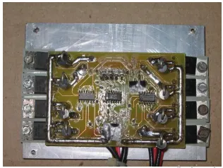
Fig. 7. Braking H-Bridge[5]
a short was found in the H-bridge. Since the H-bridge was large and also had problems with overheating in the past, it was replaced with a Pololu motor controller. The new motor
controller was chosen because it has much higher voltage and
current tolerances. The motor controller also does not require a heat sync unless using more than 15A, whereas the H-bridge
required a large heat sync just to operate at 8A. The Pololu motor controller is also much smaller, allowing it to fit in the new enclosure easily. The original H-bridge is shown in Figure
7.
B. Steering
The first steering system had severe overheating problems[2]. One of the key components of the Electric Power Steering system’s operation is the torque sensor. When a difference in the angle of the wheels and the operator’shandle bar is detected, a change in resistance is output by
the sensor. The sensor has two separate resistive components. One indicates angles to the right, while the other indicates 978-1-4799-6585-4/14/$31.00 ©2014 IEEE angles to the left. The third wire is connected to ground. A picture of this is shown in Figures 9 and 10.
From experiments using a multi-meter, the following torque sensor system function was discovered[6]:
• Pin A: W/Bu wire = Right Turn. Varies from 13W at
neutral (no steering effort) to 9.5W at maximum steering
effort (meter connected A to C).
• Pin B: Y/R wire =: Left Turn. Same specification as Pin A (connected B to C).
• Pin C: G/O wire = Ground. Continuity with Chassis.
A circuit of parallel resistors was developed with switches to add and remove resistors. PWM is used to emulate intermediate resistances. Since very low resistances were being used, Maxim ICs MAX4668 Dual SPST CMOS Analog Switch was selected to switch resistors on and off. This switch has a low
on resistance of 2.5Ω, making it ideal for this application. A US Digital MAE3 Digital Magnetic Encoder was attached to the steering column to determine the current steering angle.
The encoder is shown in Figure 11. The encoder is used for feedback in the closed loop control system. The new steering system only has overheating problems when attempting to steer while completely stationary. While stationary, the steering system is over damped, causing it to steer slowly and overheat. While moving, the over damping problems should be reduced since the motor will have less resistance from friction. During the steering redesign, the steering controller was also turned into a CAN bus node. This allowed easy integration of the steering controller into the new system. The steering control node is shown in Figures 12 and
13.
C. Remote Control
A Spektrum DX6 transmitter and a BR6000 receiver were used to control the ATV. Theses are typically used for controlling model airplanes. Since this controller is normally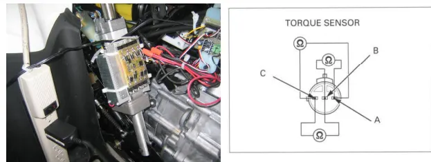
used for yaw, pitch, and roll, most of the channels were not
Fig. 8. Braking Linear Actuator[5],Fig. 9. Torque Sensor Schematic[6]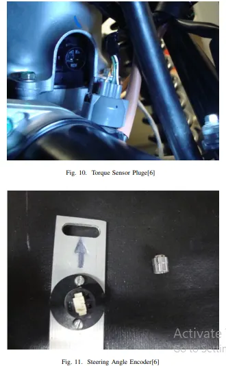
Fig. 10. Torque Sensor Pluge[6]
Fig. 11. Steering Angle Encoder[6]
978-1-4799-6585-4/14/$31.00 ©2014 IEEE
Fig. 12. Steering Control Node[6]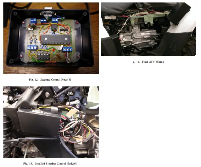
Fig. 13. Installed Steering Control Node[6],Fig. 14. Final ATV Wiring
needed. Only one of the joysticks on the controller. Forward and backwards were interpreted into acceleration or braking respectively, since the ATV cannot currently go into reverse on
its own. The RX63N microcontroller read the pulses coming from the receiver and interpreted them into commands for each of the nodes on the bus.
IV. CONCLUSION
The ATV is now fully operational using an RC transmitter. A CAN bus network has been successfully installed on board the ATV. A new control node has been developed for the steering control system. Another node was developed for controlling the throttle and brakes. The remote control functionality as well as the new steering control node have been reintegrated into the system. Also, a new master control node has been completed which takes the radio receiver’s signals and interprets them into commands across the CAN bus. The steering, throttle, and brakes can all be controlled across the CAN bus now. All of the wiring has been placed into enclosures with their respective nodes. The two new nodes are shown in Figure 14. The master control node is in the top right enclosure and the braking and throttle node is in the
bottom left.
V. FUTURE WORK
A kill switch still needs to be added to the system so that the ATV can be shut off in case of an emergency. The kill switch can also act as a simple on off switch. Currently the wiring
is disconnected whenever testing is completed and a switch would simplify this process as well as make it safer. The actuator needs some sort of feedback system to the Sakura.Currently, the Sakura works with the brake by assuming it is in the raised position at startup. Some possible options include adding an LVDT or potentiometer to the actuator. Inthe future sensors will be added to the ATV and integratedinto previous work on path planning algorithms to make it fully autonomous.
How CVTs Work
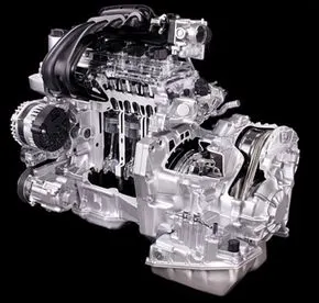
Some say you can't teach an old dog new tricks. But the continuously variable transmission (CVT), which Leonardo da Vinci conceptualized more than 500 years ago and is now replacing planetary automatic transmissions in some automobiles, is one old dog that has definitely learned a few new tricks. Indeed, ever since the first toroidal CVT patent was filed in 1886, the technology has been refined and improved. Today, several car manufacturers, including General Motors, Audi, Honda and Nissan, are designing their drivetrains around CVTs.
In this article, we'll explore how a CVT works in a typical rear-wheel driven car, answering several questions on the way:
- What parts does it have and how do those parts work?
- What advantages do CVTs offer over conventional automatic transmissions? What about disadvantages?
- What's the driving experience like in a car with a CVT?
- What kind of makes and models incorporate CVTs?
- Are there any other applications for CVTs other than automobiles?
First, we'll look at how a CVT compares to a traditional automatic transmission.
Transmission Basics
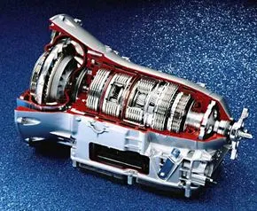
If you've read about the structure and function of automatic transmissions in How Automatic Transmissions Work, then you know that the job of the transmission is to change the speed ratio between the engine and the wheels of an automobile. In other words, without a transmission, cars would only have one gear -- the gear that would allow the car to travel at the desired top speed. Imagine for a moment driving a car that only had first gear or a car that only had third gear. The former car would accelerate well from a complete stop and would be able to climb a steep hill, but its top speed would be limited to just a few miles an hour. The latter car, on the other hand, would fly at 80 mph down the highway, but it would have almost no acceleration when starting out and wouldn't be able to climb hills.
So the transmission uses a range of gears -- from low to high -- to make more effective use of the engine's torque as driving conditions change. The gears can be engaged manually or automatically.
In a traditional automatic transmission, the gears are literally gears -- interlocking, toothed wheels that help transmit and modify rotary motion and torque. A combination of planetary gears creates all of the different gear ratios that the transmission can produce, typically four forward gears and one reverse gear. When this type of transmission cycles through its gears, the driver can feel jolts as each gear is engaged.
CVT Basics
Unlike traditional automatic transmissions, continuously variable transmissions don't have a gearbox with a set number of gears, which means they don't have interlocking toothed wheels. The most common type of CVT operates on an ingenious pulley system that allows an infinite variability between highest and lowest gears with no discrete steps or shifts.
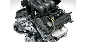
If you're wondering why the word "gear" still appears in the explanation of a CVT, remember that, broadly speaking, a gear refers to a ratio of engine shaft speed to driveshaft speed. Although CVTs change this ratio without using a set of planetary gears, they are still described as having low and high "gears" for the sake of convention.
Next, we'll look at the different types of CVTs: pulley-based, toroidal and hydrostatic.
- 1490 - da Vinci sketches a stepless continuously variable transmission
- 1886 - first toroidal CVT patent filed
- 1935 - Adiel Dodge receives U.S. patent for toroidal CVT
- 1939 - fully automatic transmission based on planetary gear system introduced
- 1958 - Daf (of The Netherlands) produces a CVT in a car
- 1989 - Subaru Justy GL is the first U.S.-sold production automobile to offer a CVT
- 2002 - Saturn Vue with a CVT debuts; first Saturn to offer CVT technology
- 2004 - Ford begins offering a CVT
Pulley-based CVTs
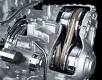
Peer into a planetary automatic transmission, and you'll see a complex world of gears, brakes, clutches and governing devices. By comparison, a continuously variable transmission is a study in simplicity. Most CVTs only have three basic components:
- A high-power metal or rubber belt
- A variable-input "driving" pulley
- An output "driven" pulley
CVTs also have various microprocessors and sensors, but the three components described above are the key elements that enable the technology to work.
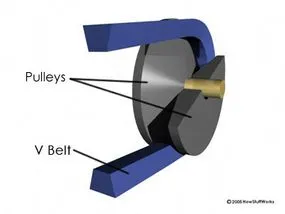
The variable-diameter pulleys are the heart of a CVT. Each pulley is made of two 20-degree cones facing each other. A belt rides in the groove between the two cones. V-belts are preferred if the belt is made of rubber. V-belts get their name from the fact that the belts bear a V-shaped cross section, which increases the frictional grip of the belt.
When the two cones of the pulley are far apart (when the diameter increases), the belt rides lower in the groove, and the radius of the belt loop going around the pulley gets smaller. When the cones are close together (when the diameter decreases), the belt rides higher in the groove, and the radius of the belt loop going around the pulley gets larger. CVTs may use hydraulic pressure, centrifugal force or spring tension to create the force necessary to adjust the pulley halves.
Variable-diameter pulleys must always come in pairs. One of the pulleys, known as the drive pulley (or driving pulley), is connected to the crankshaft of the engine. The driving pulley is also called the input pulley because it's where the energy from the engine enters the transmission. The second pulley is called the driven pulley because the first pulley is turning it. As an output pulley, the driven pulley transfers energy to the driveshaft.
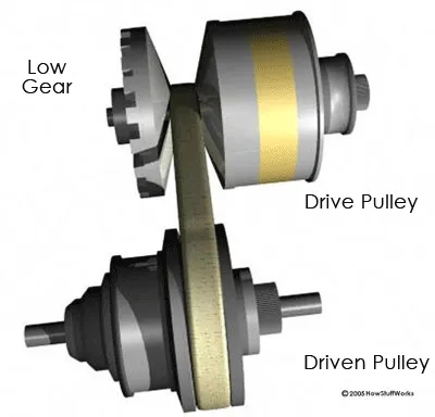
When one pulley increases its radius, the other decreases its radius to keep the belt tight. As the two pulleys change their radii relative to one another, they create an infinite number of gear ratios -- from low to high and everything in between. For example, when the pitch radius is small on the driving pulley and large on the driven pulley, then the rotational speed of the driven pulley decreases, resulting in a lower “gear.” When the pitch radius is large on the driving pulley and small on the driven pulley, then the rotational speed of the driven pulley increases, resulting in a higher “gear.” Thus, in theory, a CVT has an infinite number of "gears" that it can run through at any time, at any engine or vehicle speed.
The simplicity and stepless nature of CVTs make them an ideal transmission for a variety of machines and devices, not just cars. CVTs have been used for years in power tools and drill presses. They've also been used in a variety of vehicles, including tractors, snowmobiles and motor scooters. In all of these applications, the transmissions have relied on high-density rubber belts, which can slip and stretch, thereby reducing their efficiency.
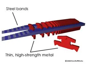
The introduction of new materials makes CVTs even more reliable and efficient. One of the most important advances has been the design and development of metal belts to connect the pulleys. These flexible belts are composed of several (typically nine or 12) thin bands of steel that hold together high-strength, bow-tie-shaped pieces of metal.
Metal belts don't slip and are highly durable, enabling CVTs to handle more engine torque. They are also quieter than rubber-belt-driven CVTs.
Toroidal CVTs
Another version of the CVT -- the toroidal CVT system -- replaces the belts and pulleys with discs and power rollers.
Although such a system seems drastically different, all of the components are analogous to a belt-and-pulley system and lead to the same results -- a continuously variable transmission. Here's how it works:
- One disc connects to the engine. This is equivalent to the driving pulley.
- Another disc connects to the drive shaft. This is equivalent to the driven pulley.
- Rollers, or wheels, located between the discs act like the belt, transmitting power from one disc to the other.
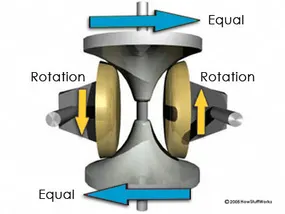
The wheels can rotate along two axes. They spin around the horizontal axis and tilt in or out around the vertical axis, which allows the wheels to touch the discs in different areas. When the wheels are in contact with the driving disc near the center, they must contact the driven disc near the rim, resulting in a reduction in speed and an increase in torque (i.e., low gear). When the wheels touch the driving disc near the rim, they must contact the driven disc near the center, resulting in an increase in speed and a decrease in torque (i.e., overdrive gear). A simple tilt of the wheels, then, incrementally changes the gear ratio, providing for smooth, nearly instantaneous ratio changes.
Hydrostatic CVTs
Both the pulley-and-V-belt CVT and the toroidal CVT are examples of frictional CVTs, which work by varying the radius of the contact point between two rotating objects. There is another type of CVT, known as a hydrostatic CVT, that uses variable-displacement pumps to vary the fluid flow into hydrostatic motors. In this type of transmission, the rotational motion of the engine operates a hydrostatic pump on the driving side. The pump converts rotational motion into fluid flow. Then, with a hydrostatic motor located on the driven side, the fluid flow is converted back into rotational motion.
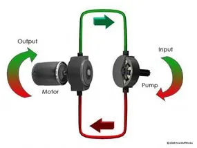
Often, a hydrostatic transmission is combined with a planetary gearset and clutches to create a hybrid system known as a hydromechanical transmission. Hydromechanical transmissions transfer power from the engine to the wheels in three different modes. At a low speed, power is transmitted hydraulically, and at a high speed, power is transmitted mechanically. Between these extremes, the transmission uses both hydraulic and mechanical means to transfer power. Hydromechanical transmissions are ideal for heavy-duty applications, which is why they are common in agricultural tractors and all-terrain vehicles.
CVT Benefits
Continuously variable transmissions are becoming more popular for good reason. They boast several advantages that make them appealing both to drivers and to environmentalists. Here are some of the key features and benefits of CVTs:
Features
- Constant, stepless acceleration from a complete stop to cruising speed
- Works to keep the car in its optimum power range regardless of how fast the car is traveling
- Responds better to changing conditions, such as changes in throttle and speed
- Less power loss in a CVT than a typical automatic transmission
- Better control of a gasoline engine's speed range
- Can incorporate automated versions of mechanical clutches
Benefits
- Eliminates "shift shock" -- makes for a smoother ride
- Improved fuel efficiency
- Eliminates gear hunting as a car decelerates, especially going up a hill
- Better acceleration
- Better control of emissions
- Replace inefficient fluid torque converter
In the next section, we'll look at what it's like to drive a CVT-based car.
A CVT Test Drive
Cars with CVTs have been common in Europe for years. But it's taken a while for the technology to gain a foothold in the United States. The first production automobile to offer a CVT in the United States was the Subaru Justy.
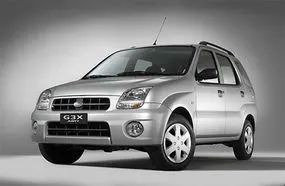
Sold between 1989 and 1993, the Justy never attracted the attention of American drivers. So what's different about newer CVT-based cars -- cars like the Saturn Vue, the Audi A4 and A6, the Nissan Murano and the Honda Insight? The best way to answer that question is to take one of these cars for a test drive.
When you step on the gas pedal of a car with a continuously variable transmission, you notice the difference immediately. The engine revs up toward the rpms at which it produces the most power, and then it stays there. But the car doesn't react immediately. Then, a moment later, the transmission kicks in, accelerating the car slowly, steadily and without any shifts. In theory, a car with a CVT should reach 60 mph (100 km/hr) 25-percent faster than the same car with the same engine and a manual transmission [ref]. That's because the CVT converts every point on the engine's operating curve to a corresponding point on its own operating curve.
If you look at the power output curve for the car without a CVT, you can see this to be true. Notice that the tachometer in this situation shows the engine revving up and down with each gear change, which is recorded as a spike in the power output curve (and which the driver feels as a jolt).
CVTs are equally efficient on hills. There is no "gear hunting," because the CVT cycles steplessly down to a gear ratio appropriate for the driving conditions. A conventional automatic transmission shifts back and forth trying to find the right gear, which is far less efficient.
With all of their advantages, CVTs do have some shortcomings. In the United States, they are still trying to overcome an image problem. The Subaru Justy, for example, was known as a gutless micro-car. Traditionally, belt-drive CVTs were limited in the amount of torque they could handle and were larger and heavier than their automatic and manual counterparts. Technological advances have put CVTs in the realm of their competition -- the Nissan Murano's CVT can handle its 3.5-liter, 245-horsepower V6 engine -- but first impressions are hard to overcome.
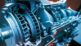
IN MATLAB/SIMULINK the simulation of baja atv is done and components along with the results are explained below:
Components used:
Signal Builder
Create and generate interchangeable groups of signals whose waveforms are piecewise linearexpand all in page
Library:
Simulink / Sources
Description
The Signal Builder block allows you to create interchangeable groups of piecewise linear signal sources and use them in a model. You can quickly switch the signal groups into and out of a model to facilitate testing. In the Signal Builder window, create signals and define the output waveforms.To open the window, double-click the block. See Signal Groups.
Note
Use the signalbuilder function to create and access Signal Builder blocks programmatically.
Ports
Output
collapse all
Signal 1 — First output signal
scalar | vector | matrix
First output signal from the signal group currently visible in the Signal Builder window.
Data Types: double | bus
Signal n — nth output signal
scalar | vector | matrix
nth output signal from the signal group currently visible in the Signal Builder window. n corresponds to the signal index.
Data Types: double | bus
Block Characteristics
Data Types double
Direct Feedthrough No
Multidimensional Signals No
Variable-Size Signals No
Zero-Crossing Detection Yes
Generic Engine
Internal combustion engine with throttle and rotational inertia and time lag
Library
Simscape / Driveline / Engines
Description
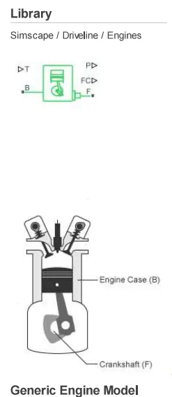
The Generic Engine block represents a general internal combustion engine. Engine types include spark-ignition and diesel. Speed-power and speed-torque parameterizations are provided. A throttle physical signal input specifies the normalized engine torque. Optional dynamic parameters include crankshaft inertia and response time lag. A physical signal port outputs engine fuel consumption rate based on choice of fuel consumption model. Optional speed and redline controllers prevent engine stall and enable cruise control.
Generic Engine Model
By default, the Generic Engine model uses a programmed relationship between torque and speed, modulated by the throttle signal.
Engine Speed, Throttle, Power, and Torque
The engine model is specified by an engine power demand function g(Ω). The function provides the maximum power available for a given engine speed Ω. The block parameters (maximum power, speed at maximum power, and maximum speed) normalize this function to physical maximum torque and speed values.
The normalized throttle input signal T specifies the actual engine power. The power is delivered as a fraction of the maximum power possible in a steady state at a fixed engine speed. It modulates the actual power delivered, P, from the engine: P(Ω,T) = T·g(Ω). The engine torque is τ = P/Ω.
Engine Power Demand
The engine power is nonzero when the speed is limited to the operating range, Ωmin ≤ Ω ≤ Ωmax. The absolute maximum engine power Pmax defines Ω0 such that Pmax = g(Ω0). Define w ≡ Ω/Ω0 and g(Ω) ≡ Pmax·p(w). Then p(1) = 1 and dp(1)/dw = 0. The torque function is:
τ = (Pmax/Ω0)·[p(w)/w].
You can derive forms for p(w) from engine data and models. Generic Engine uses a third-order polynomial form:
p(w) = p1·w + p2·w2 – p3·w3
satisfying
p1 + p2 – p3 = 1, p1 + 2p2 – 3p3 = 0.
In typical engines, the pi are positive. This polynomial has three zeros, one at w = 0, and a conjugate pair. One of the pair is positive and physical; the other is negative and unphysical:
Typical Engine Power Demand Function
Restrictions on Engine Speed and Power
For the engine power polynomial, there are restrictions, as shown, on the polynomial coefficients pi, to achieve a valid power-speed curve.
If you use tabulated power or torque data, corresponding restrictions on P(Ω) remain.
Specify the speed and power as w = Ω/Ω0 and p = P(Ω)/P0 and define the boundaries as wmin = Ωmin/Ω0 and wmax = Ωmax/Ω0. Then:
The engine speed is restricted to a positive range above the minimum speed and below the maximum speed: 0 ≤ wmin ≤ w ≤ wmax.
The engine power at minimum speed must be nonnegative: p(wmin) ≥ 0. If you use the polynomial form, this condition is a restriction on the pi:
p(wmin) = p1·wmin + p2·w2min – p3·wmin3 ≥ 0.
The engine power at maximum speed must be nonnegative: p(wmax) ≥ 0. If you use the polynomial form, this condition is a restriction on wmax: wmax ≤ w+.
Engine Power Forms for Different Engine Types
For the default parameterization, Generic Engine provides two choices of internal combustion engine types, each with different engine power demand parameters.
Power Demand
Coefficient Engine Type:
Spark-Ignition Diesel
p1 1 0.6526
p2 1 1.6948
p3 1 1.3474
Idle Speed Controller Model
The idle speed controller adjusts the throttle signal to increase engine rotation below a reference speed according to the following expressions:
Π=max(Πi ,Πc)
and
d(Πc)dt =0.5⋅(−tanh(4⋅ω−ωrω))−Πcτ
where:
Π — Engine throttle
Πi — Input throttle (port T)
Πc — Controller throttle
ω — Engine speed
ωr — Idle speed reference
ωt — Controller speed threshold
τ — Controller time constant
The controlled throttle increases with a first-order lag from zero to one when engine speed falls below the reference speed. When the engine speed rises above the reference speed, the controlled throttle decreases from one to zero. When the difference between engine velocity and reference speed is smaller than the controller speed threshold, the tanh function smooths the time derivative of the controlled throttle. The controlled throttle is limited to the range 0–1. The engine uses the larger of the input and controlled throttle values. If engine time lag is included, the controller changes the input before the lag is computed.
Redline Controller Model
While the idle speed controller determines the minimum throttle value for maintaining engine speed, the redline controller prevents excessive speed based on a maximum throttle input. To determine the maximum throttle value, the redline controller uses the idle speed controller model equation. However, for the redline controller:
ωr is the redline speed reference.
ωt is the redline speed threshold.
τ is the redline time constant.
Performance
To increase simulation speed, use the default option, No fuel consumption, for the Fuel consumption model parameter.
If you select any other option for the Fuel consumption model, the block solves a nonlinear equation that is required for calculating fuel consumption. The block solves the equation even if the FC port, which reports the fuel consumption rate, is not connected to another block.
When the parameter is set to No fuel consumption, the block does not calculate fuel consumption, even if the FC port is connected to another block.
Limitations
This block contains an engine time lag limitation.
Engine Time Lag
Engines lag in their response to changing speed and throttle. The Generic Engine block optionally supports lag due to a changing throttle only. Time lag simulation increases model fidelity but reduces simulation performance.
Ports
Port Description
B Rotational conserving port representing the engine block
F Rotational Conserving port representing the engine crankshaft
T Physical signal input port specifying the normalized engine throttle level
P Physical signal output port reporting the instantaneous engine power
FC Physical signal output port reporting the fuel consumption rate
Port T accepts a signal with values in the range 0–1. The signal specifies the engine torque as a fraction of the maximum torque possible in steady state at fixed engine speed. The signal saturates at zero and one. Values below zero are interpreted as zero. Values above one are interpreted as one.
Port FC does not output data when the Fuel consumption model parameter is set to No fuel consumption.
Parameters
Engine Torque
The table shows how the visibility of some parameters depends on the option that you choose for other parameters. To learn how to read the table, see Parameter Dependencies.
Engine Torque Parameter Dependencies
Engine Torque
Model parameterization — Choose Normalized 3rd-order polynomial matched to peak power, Tabulated torque data, or Tabulated power data
Normalized 3rd-order polynomial matched to peak power Tabulated torque data Tabulated power data
Engine type — Choose Spark-ignition or Diesel
Speed vector
Maximum power
Torque vector
Speed at maximum power
Interpolation method — Choose Linear or Smooth
Maximum speed
Stall speed
Model parameterization
Select how to model the engine. Choose between these options, each of which enable other parameters:
Normalized 3rd-order polynomial matched to peak power — Parametrize the engine with a power function controlled by power and speed characteristics. This is the default option.
Tabulated torque data — Engine is parametrized by speed–torque table that you specify.
Tabulated power data — Engine is parametrized by speed–power table that you specify.
Engine type
Choose type of internal combustion engine. Choose between Spark-ignition, the default option, and Diesel.
Selecting Normalized 3rd-order polynomial matched to peak power for the Model parameterization parameter exposes this parameter.
For more information, see the Engine Torque Parameter Dependencies table.
Maximum power
Maximum power Pmax that the engine can output. The default is 150 kW.
Selecting Normalized 3rd-order polynomial matched to peak power for the Model parameterization parameter exposes this parameter.
For more information, see the Engine Torque Parameter Dependencies table.
Speed at maximum power
Engine speed Ω0 at which the engine is running at maximum power. The default is 4500 rpm.
Selecting Normalized 3rd-order polynomial matched to peak power for the Model parameterization parameter exposes this parameter.
For more information, see the Engine Torque Parameter Dependencies table.
Maximum speed
Maximum speed Ωmax at which the engine can generate torque. The default is 6000 rpm.
During simulation, if Ω exceeds this maximum, the simulation stops with an error. The engine maximum speed Ωmax cannot exceed the engine speed at which the engine power becomes negative.
Selecting Normalized 3rd-order polynomial matched to peak power for the Model parameterization parameter exposes this parameter.
For more information, see the Engine Torque Parameter Dependencies table.
Stall speed
Minimum speed Ωmin at which the engine can generate torque. The default is 500 rpm.
During simulation, if Ω falls below this minimum, the engine torque is blended to zero.
Selecting Normalized 3rd-order polynomial matched to peak power for the Model parameterization parameter exposes this parameter.
For more information, see the Engine Torque Parameter Dependencies table.
Speed vector
Vector of values of the engine function's independent variable, the speed Ω. The default is [500, 1000, 2000, 3000, 4000, 5000, 6000, 7000] rpm.
The first and last speeds in the vector are interpreted as the stall speed and the maximum speed, respectively. If the speed falls below the stall speed, engine torque is blended to zero. If the speed exceeds the maximum speed, the simulation stops with an error.
Selecting Tabulated torque data or Tabulated power data for the Model parameterization parameter exposes this parameter.
For more information, see the Engine Torque Parameter Dependencies table.
Torque vector
Vector of values of the engine function's dependent variable, the torque τ. The default is [380, 380, 380, 380, 350, 280, 200, 80] N*m.
Selecting Tabulated torque data for the Model parameterization parameter exposes this parameter.
For more information, see the Engine Torque Parameter Dependencies table.
Power vector
Vector of values of the engine function's dependent variable, the power P. The default is [20, 40, 78, 120, 145, 148, 125, 60] kW.
Selecting Tabulated power data for the Model parameterization parameter exposes this parameter.
For more information, see the Engine Torque Parameter Dependencies table.
Interpolation method
Method to interpolate the engine speed–torque or speed–power function between discrete relative velocity values within the range of definition. Choose between Linear, the default choice, and Smooth.
Selecting Tabulated torque data or Tabulated power data for the Model parameterization parameter exposes this parameter.
For more information, see the Engine Torque Parameter Dependencies table.
Dynamics
The table shows how the visibility of some parameters depends on the option that you choose for other parameters. To learn how to read the table, see Parameter Dependencies.
Dynamics Parameter Dependencies
Dynamics
Inertia — Choose No inertia or Specify inertia and initial velocity
No inertia Specify inertia and initial velocity
Engine inertia
Initial velocity
Time constant — Choose No lag - Suitable for HIL simulation or Specify time constant and initial value
No lag - Suitable for HIL simulation Specify time constant and initial value
Engine time constant
Initial normalized throttle
Inertia
Select how to model the rotational inertia of the engine block. Choose between these options, each of which exposes other parameters:
No inertia — Engine crankshaft is modeled with no inertia. This option is the default.
Specify inertia and initial velocity — Engine crankshaft is modeled with rotational inertia and initial angular velocity.
Engine Inertia
Rotational inertia of the engine crankshaft. The default is 1 kg*m^2.
Selecting Specify inertia and initial velocity for the Inertia parameter exposes this parameter.
For more information, see the Dynamics Parameter Dependencies table.
Initial velocity
Initial angular velocity Ω(0) of the engine crankshaft. The default is 800 rpm.
Selecting Specify inertia and initial velocity for the Inertia parameter exposes this parameter.
For more information, see the Dynamics Parameter Dependencies table.
Time constant
Select how to model the time lag of the engine response. Choose between these options, each of which exposes other options:
No lag — Suitable for HIL simulation — Engine reacts with no time lag. This option is the default.
Specify time constant and initial value — Engine reacts with a time lag.
Selecting Specify time constant and initial value exposes other parameters.
For more information, see the Dynamics Parameter Dependencies table.
Engine time constant
Engine time lag. The default is 0.2 s.
Selecting Specify time constant and initial value for the Time constant parameter exposes this parameter.
For more information, see the Dynamics Parameter Dependencies table.
Initial normalized throttle
Initial normalized engine throttle T(0), ranging between zero and one. The default is 0.
Selecting Specify time constant and initial value for the Time constant parameter exposes this parameter.
For more information, see the Dynamics Parameter Dependencies table.
Limits
Speed threshold
Width of the speed range over which the engine torque is blended to zero as Ω approaches the stall speed. The default is 100 rpm.
Fuel Consumption
The table shows how the visibility of some parameters depends on the option that you choose for other parameters. To learn how to read the table, see Parameter Dependencies.
Fuel Consumption Parameter Dependencies
Fuel Consumption
Fuel consumption model — Choose No fuel consumption, Constant per revolution, Fuel consumption by speed and torque, Brake specific fuel consumption by speed and torque, or Brake specific fuel consumption by speed and brake mean effective pressure
No fuel consumption Constant per revolution Fuel consumption by speed and torque Brake specific fuel consumption by speed and torque Brake specific fuel consumption by speed and brake mean effective pressure
Fuel consumption per revolution
Displaced volume
Revolutions per cycle
Speed vector
Torque vector
Brake mean effective pressure vector
Fuel consumption table
Brake specific fuel consumption table
Interpolation method — Choose Linear or Smooth
Fuel consumption model
Select a model for calculating engine-fuel consumption. Model parameterizations are compatible with standard industrial data. Choose between these options:
No fuel consumption — The default option
Constant per revolution
Fuel consumption by speed and torque
Brake specific fuel consumption by speed and torque
Brake specific fuel consumption by speed and brake mean effective pressure
Some options expose other parameters. For more information, see the Fuel Consumption Parameter Dependencies table.
No fuel consumption
The block does not calculate fuel consumption even when the FC port, which reports the fuel consumption rate, is connected to another block. Selecting this option increases simulation speed.
Fuel consumption per revolution
Enter the volume of fuel consumed in one crankshaft revolution. The default is 25 mg/rev.
Selecting Constant per revolution for the Fuel consumption model parameter exposes this parameter.
For more information, see the Fuel Consumption Parameter Dependencies table.
Displaced volume
Enter the volume displaced by a piston stroke. The default is 400 cm^3.
Selecting Brake specific fuel consumption by speed and brake mean effective pressure for the Fuel consumption model parameter exposes this parameter.
For more information, see the Fuel Consumption Parameter Dependencies table.
Revolutions per cycle
Enter the number of crankshaft revolutions in one combustion cycle — e.g. 2 for a four-stroke engine, or 1 for a two-stroke engine. The default is 2.
Selecting Brake specific fuel consumption by speed and brake mean effective pressure for the Fuel consumption model parameter exposes this parameter.
For more information, see the Fuel Consumption Parameter Dependencies table.
Speed vector
Enter vector of engine speeds used in lookup table parameterizations. Vector size must match Torque vector size. The default is [1000, 2000, 3000, 4000, 5000, 6000] rpm. Selecting Fuel consumption by speed and torque, Brake specific fuel consumption by speed and torque, or Brake specific fuel consumption by speed and brake mean effective pressure for the Fuel consumption model parameter exposes this parameter.
For more information, see the Fuel Consumption Parameter Dependencies table.
Torque vector
Enter vector of engine torques used in the lookup table parameterizations. Vector size must match Speed vector size. The default is [0, 80, 160, 200, 240, 320, 360, 400] N*m. Selecting Fuel consumption by speed and torque or Brake specific fuel consumption by speed and torque for the Fuel consumption model parameter exposes this parameter.
For more information, see the Fuel Consumption Parameter Dependencies table.
Fuel consumption table
Enter matrix with fuel consumption rates corresponding to engine speed and torque vectors. The number of rows must equal the number of elements in the Speed vector. The number of columns must equal the number of elements in the Torque vector. The default is [.5, .9, 1.4, 1.6, 1.9, 2.7, 3.4, 4.4; 1, 1.7, 2.7, 3.1, 3.6, 5, 6, 7.4; 1.4, 2.7, 4, 4.8, 5.6, 7.5, 8.5, 10.5; 2, 3.6, 5.8, 6.7, 8, 10.4, 11.7, 13.3; 2.5, 4.8, 7.9, 9.4, 10.8, 14, 16.2, 18.6; 3.1, 6, 10.3, 11.9, 13.8, 18.4, 22, 26.5] g/s.
Selecting Fuel consumption by speed and torque for the Fuel consumption model parameter exposes this parameter.
For more information, see the Fuel Consumption Parameter Dependencies table.
Brake mean effective pressure vector
Enter vector of brake mean effective pressure (BMEP) values. The default is [0, 250, 500, 625, 750, 1000, 1150, 1250] kPa. The BMEP satisfies the expression:
BMEP=T⋅(2π⋅ncVd)
where:T — Output torque
nc — Number of cycles per revolution
Vd — Cylinder displaced volume
Selecting Brake specific fuel consumption by speed and brake mean effective pressure for the Fuel consumption model parameter exposes this parameter.
For more information, see the Fuel Consumption Parameter Dependencies table.
Brake specific fuel consumption table
Selecting Brake specific fuel consumption by speed and torque or Brake specific fuel consumption by speed and brake mean effective pressure for the Fuel consumption model parameter exposes this parameter.
For more information, see the Fuel Consumption Parameter Dependencies table.
For the Brake specific fuel consumption by speed and torque fuel model, enter the matrix with brake specific fuel consumption (BSFC) rates corresponding to engine speed and torque vectors. BSFC is the ratio of the fuel consumption rate to the output power. The number of rows must equal the number of elements in the Speed vector. The number of columns must equal the number of elements in the Torque vector.
For the Brake specific fuel consumption by speed and brake mean effective pressure fuel model, enter the matrix with brake specific fuel consumption (BSFC) rates corresponding to engine speed and brake mean effective pressure (BMEP) vectors. BSFC is the ratio of the fuel consumption rate to the output power. The number of rows must equal the number of elements in the Speed vector. The number of columns must equal the number of elements in the Brake mean effective pressure vector.
For both fuel-consumption models, the default is [410, 380, 300, 280, 270, 290, 320, 380; 410, 370, 290, 270, 260, 270, 285, 320; 415, 380, 290, 275, 265, 270, 270, 300; 420, 390, 310, 290, 285, 280, 280, 285; 430, 410, 340, 320, 310, 300, 310, 320; 450, 430, 370, 340, 330, 330, 350, 380] g/hr/kW.
Interpolation method
Select the interpolation method used to calculate fuel consumption at intermediate speed-torque values. Methods are Linear and Smooth. Outside the data range, fuel consumption is held constant at the last value given in the lookup table. Selecting Fuel consumption by speed and torque, Brake specific fuel consumption by speed and torque, or Brake specific fuel consumption by speed and brake mean effective pressure for the Fuel consumption model parameter exposes this parameter.
For more information, see the Fuel Consumption Parameter Dependencies table.
Speed Control
The table shows how the visibility of some parameters depends on the option that you choose for other parameters. To learn how to read the table, see Parameter Dependencies.
Speed Control Parameter Dependencies
Speed Control
Idle speed control — Choose Off or On
Off On
Idle speed reference
Controller time constant
Redline control
Redline control — Choose Off or On
Off On
Redline speed
Redline time constant
Redline threshold speed
Idle speed control
Select speed control model. The options are:
Off — Omit idle speed controller. Throttle input is used directly. This option is the default.
On — Include idle speed controller to prevent engine stalling. This option exposes other parameters. For more information, see Idle Speed Controller Model.
Idle speed reference
Enter the value of the speed reference below which speed increases, and above which speed decreases. The default is 1000 rpm.
Selecting On for the Idle speed control parameter exposes this parameter.
For more information, see the Speed Control Parameter Dependencies table.
Controller time constant
Enter the value of the time constant associated with an increase or decrease of the controlled throttle. The constant value must be positive. The default is 1 s.
Selecting On for the Idle speed control parameter exposes this parameter.
For more information, see the Speed Control Parameter Dependencies table.
Controller threshold speed
Parameter used to smooth the controlled throttle value when the engine’s rotational speed crosses the idle speed reference. For more information, see Idle Speed Controller Model. Large values decrease controller responsiveness. Small values increase computational cost. This parameter must be positive. The default is 1 rpm.
Selecting On for the Idle speed control parameter exposes this parameter.
For more information, see the Speed Control Parameter Dependencies table.
Redline control
Select redline control model. Options include Off and On.
Off — Omit redline controller. Throttle depends only on the idle speed controller. This option is the default.
On — Include redline controller to prevent excessive speed. This option exposes other parameters.
For more information, see the Speed Control Parameter Dependencies table.
Redline speed
Enter the value of the speed reference above which the redline control activates. The default is 5000 rpm.
Selecting On for the Redline control parameter exposes this parameter.
For more information, see the Speed Control Parameter Dependencies table.
Redline time constant
Enter the value of the time constant associated with an increase or decrease of the controlled throttle. The constant value must be positive. The default is 1 s.
Selecting On for the Redline control parameter exposes this parameter.
For more information, see the Speed Control Parameter Dependencies table.
Redline threshold speed
Specify the width of the region around the redline speed where the controller goes from fully enabled to not enabled. The block uses this parameter for smoothing the controlled throttle value when the engine’s rotational speed crosses the redline speed reference. Large values decrease controller responsiveness. Small values increase computational cost. This parameter must be positive. The default is 1 rpm.
Selecting On for the Redline control parameter exposes this parameter.
Ideal Rotational Motion Sensor
Motion sensor in mechanical rotational systems
- Library:
-
Simscape / Foundation Library / Mechanical / Mechanical Sensors

Description
The Ideal Rotational Motion Sensor block represents an ideal mechanical rotational motion sensor, that is, a device that converts an across variable measured between two mechanical rotational nodes into a control signal proportional to angular velocity or angle. You can specify the initial angular position (offset) as a block parameter.
The sensor is ideal since it does not account for inertia, friction, delays, energy consumption, and so on.
Connections R and C are mechanical rotational conserving ports that connect the block to the nodes whose motion is being monitored. Connections W and A are physical signal output ports for velocity and angular displacement, respectively.
The block positive direction is from port R to port C. This means that the velocity is measured as ω = ωR – ωC, where ωR, ωC are the absolute angular velocities at ports R and C, respectively.
Ports
Output
W — Angular velocity, rad/s
physical signal
Physical signal output port for angular velocity.
A — Angular displacement, rad
physical signal
Physical signal output port for angular displacement.
Conserving
R — Rod (positive probe)
mechanical rotational
Mechanical rotational conserving port associated with the sensor positive probe.
C — Case (reference probe)
mechanical rotational
Mechanical rotational conserving port associated with the sensor negative (reference) probe.
Parameters
Initial angle — Sensor initial offset
0 rad (default)
Variable Ratio Transmission
Dynamic gearbox with variable and controllable gear ratio, transmission compliance, and friction losses
Library
Simscape / Driveline / Couplings & Drives
Description
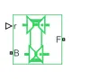
The Variable Ratio Transmission block represents a gearbox that dynamically transfers motion and torque between the two connected driveshaft axes, base and follower.
Ignoring the dynamics of transmission compliance, the driveshafts are constrained to corotate with a variable gear ratio that you control. You can choose whether the follower axis rotates in the same or opposite direction as the base axis. If they rotate in the same direction, ωF and ωB have the same sign. If they rotate in opposite directions, ωF and ωB have opposite signs.
Transmission compliance introduces internal time delay between the axis motions. Therefore, unlike a gear, a variable ratio transmission does not act as a kinematic constraint. You can also control torque loss caused by transmission and viscous losses.
Ports
B and F are rotational conserving ports representing, respectively, the base and follower driveshafts.
You specify the unitless variable gear ratio gFB(t) as a function of time at the physical signal input at port r. If the signal value becomes zero or negative, the simulation stops with an error.
Variable Ratio Transmission Model
Ideal Motion and Torque Transfer
Variable Ratio Transmission is a dynamical mechanism for transferring motion and torque between base and follower.
If the relative compliance ϕ between the axes is absent, the block is equivalent to a gear with a variable ratio gFB(t). Such a gear imposes a time-dependent kinematic constraint on the motions of the two driveshafts:
ωB = ±gFB(t)·ωF , τF = ±gFB(t)·τB .
However, Variable Ratio Transmission does include compliance between the axes. Dynamical motion and torque transfer replace the kinematic constraint, with a nonzero ϕ that dynamically responds through base compliance parameters kp and kv:
dϕ/dt = ±gFB(t)·ωF – ωB ,
τB = –kpϕ – kvdϕ/dt ,
±gFB(t)·τB + τF – τloss = 0 .
τloss = 0 in the ideal case.
Estimating Compliance Parameters
-
You can estimate the base angular compliance kp from the transmission time constant tc and inertia J: kp = J(2π/tc)2.
-
You can estimate the base angular velocity compliance kv from the transmission time constant tc, inertia J, and damping coefficient C: kv = (2Ctc)/2π = 2C√(J/kp).
Nonideal Torque Transfer and Losses
With nonideal torque transfer, τloss ≠ 0. Losses in the Variable Ratio Transmission are modeled similarly to how losses are modeled in nonideal gears. For general information on nonideal gear modeling.
In a nonideal gearbox, the angular velocity and compliance dynamics are unchanged. The transferred torque and power are reduced by:
-
Coulomb friction (for example, between belt and wheel, or internal belt losses due to stretching) characterized by an efficiency η.
-
Viscous coupling of driveshafts with bearings, parametrized by viscous friction coefficients μ.
τloss = τCoul·tanh(4ωout/ωth) + μBωB + μFωF , τCoul = |τF|·(1 – η) .
When the angular velocity changes sign, the hyperbolic tangent regularizes the sign change in the Coulomb friction torque.
| Power Flow | Power Loss Condition | Output Driveshaft ωout |
|---|---|---|
| Forward | ωBτB > ωFτF | Follower, ωF |
| Reverse | ωBτB < ωFτF | Base, ωB |
Meshing Efficiency
The friction loss represented by efficiency η is fully applied only if the absolute value of the follower angular velocity ωF is greater than a velocity threshold ωth.
If this absolute velocity is less than ωth, the actual efficiency is automatically regularized to one at zero velocity.
Parameters
Main
- Output shaft rotates
-
From the drop-down list, choose how the output driveshaft rotates relative to the input driveshaft. The default is
In same direction as input shaft.
Compliance
- Transmission stiffness at base (B)
-
Reciprocal of transmission angular compliance kp, angular displacement per unit torque, measured at the base. The default is
30000.From the drop-down list, choose units. The default is newton-meters/radian (
N*m/rad). - Transmission damping at base (B)
-
Reciprocal of transmission angular compliance damping kv, angular speed per unit torque, measured at the base. The default is
0.05.From the drop-down list, choose units. The default is newton-meters/(radian/second) (
N*m/(rad/s)). - Initial input torque at base (B)
-
Torque applied at the base driveshaft at the start of simulation (t = 0). The default is
0.From the drop-down list, choose units. The default is newton-meters (
N*m).
Transmission Losses
- Losses model
-
Select how to implement friction losses from nonideal torque transfer. The default is
No losses.-
No losses — Suitable for HIL simulation— Torque transfer is ideal. -
Constant efficiency— Transfer of torque across gearbox is reduced by a constant efficiency η satisfying 0 < η ≤ 1. If you select this option, the panel changes from its default.
-
- Viscous friction coefficients at base (B) and follower (F)
-
Vector of viscous damping coefficients [μB μF] applied at the base and follower driveshafts, respectively. The default is
[ 0 0 ].From the drop-down list, choose units. The default is newton-meters/(radian/second) (
N*m/(rad/s)).
Inertia
Ideal mechanical rotational inertia
Library
Mechanical Rotational Elements

Description
The Inertia block represents an ideal mechanical rotational inertia, described with the following equation:
T=Jdωdt
where
T |
Inertia torque |
J |
Inertia |
| ω | Angular velocity |
t |
Time |
The block has one mechanical rotational conserving port. The block positive direction is from its port to the reference point. This means that the inertia torque is positive if inertia is accelerated in positive direction.
Variables
To set the priority and initial target values for the block variables prior to simulation, use the Variables tab in the block dialog box (or the Variables section in the block Property Inspector).
- Inertia
-
Inertia. The default value is
0.001kg*m^2.
Ports
The block has one mechanical rotational conserving port, associated with the inertia connection to the system.
Simple Gear
Simple gear of base and follower wheels with adjustable gear ratio, friction losses, and triggered faults
- Library:
-
Simscape / Driveline / Gears

Description
The Simple Gear block represents a gearbox that constrains the connected driveline axes of the base gear, B, and the follower gear, F, to corotate with a fixed ratio that you specify. You choose whether the follower axis rotates in the same or opposite direction as the base axis. If they rotate in the same direction, the angular velocity of the follower, ωF, and the angular velocity of the base, ωB, have the same sign. If they rotate in opposite directions, ωF and ωB have opposite signs.
Ideal Gear Constraint and Gear Ratio
The kinematic constraint that the Simple Gear block imposes on the two connected axes is
rFωF=rBωB
where:
-
rF is the radius of the follower gear.
-
ωF is the angular velocity of the follower gear.
-
rB is the radius of the base gear.
-
ωB is the angular velocity of the base gear.
The follower-base gear ratio is
gFB=rFrB=NFNB
where:
-
NB is the number of teeth in the base gear.
-
NBF is the number of teeth in the follower gear.
Reducing the two degrees of freedom to one independent degree of freedom yields the torque transfer equation
gFBτB+τF−τloss=0
where:
-
τB is the input torque.
-
τF is the output torque.
-
τloss is the torque loss due to friction.
For the ideal case, τloss=0.
Nonideal Gear Constraint and Losses
In the nonideal case, τloss≠0. For general considerations on nonideal gear modeling,
In a nonideal gear pair (B,F), the angular velocity, gear radii, and gear teeth constraints are unchanged. But the transferred torque and power are reduced by:
-
Coulomb friction between teeth surfaces on gears B and F, characterized by efficiency, η
-
Viscous coupling of driveshafts with bearings, parametrized by viscous friction coefficients, μ
Constant Efficiency
In the constant efficiency case, η is constant, independent of load or power transferred.
Load-Dependent Efficiency
In the load-dependent efficiency case, η depends on the load or power transferred across the gears. For either power flow,
τCoul=gFBτidle+kτF
where:
-
τCoul is the Coulomb friction dependent torque.
-
k is a proportionality constant.
-
τidle is the net torque acting on the input shaft in idle mode.
Efficiency, η, is related to τCoul in the standard, preceding form but becomes dependent on load:
η=τFgFBτidle+(k+1)τF
Faults
If you enable faults for the block, the efficiency changes in response to one or both of these triggers:
-
Simulation time — A fault occurs at a specified time.
-
Simulation behavior — A fault occurs in response to an external trigger. Enabling an external fault trigger exposes port T.
If a fault trigger occurs, for the remainder of the simulation, the block uses the faulted efficiency in one of these ways:
-
Throughout rotation
-
When the rotation angle is within a faulted range that you specify
You can program the block to issue a fault report as a warning or error message.
Thermal Model
You can model the effects of heat flow and temperature change by selecting a thermal block variant. Selecting a thermal variant:
-
Exposes port H, a conserving port in the thermal domain.
-
Enables the Thermal mass parameter, which allows you to specify the ability of the component to resist changes in temperature.
-
Enables the Initial Temperature parameter, which allows you to set the initial temperature.
To select a thermal variant, right-click the block in your model and, from the context menu, select Simscape > Block choices. Select a variant that includes a thermal port.
Assumptions
-
Gear inertia is assumed negligible.
-
Gears are treated as rigid components.
-
Coulomb friction slows down simulation.
Ports
Input
T — External fault trigger
physical signal
Physical signal input port for an external fault trigger.
Dependencies
To expose the T port:
-
For the Meshing Losses Friction model parameter, select
Constant efficiencyorLoad-dependent efficiency. -
For the Faults Enable faults parameter, select
On. -
For the Faults Enable external fault trigger parameter, select
On. -
Click OK or Apply.
For information on related dependencies, .
Conserving
B — Base
rotational mechanical
Rotational mechanical conserving port associated with the base, or input, shaft.
F — Follower
rotational mechanical
Rotational mechanical conserving port associated with the follower, or output, shaft.
H — Heat
thermal
Thermal port associated with heat flow. Heat flow affects gear temperature, and therefore, power transmission efficiency.
Dependencies
The thermal conserving port is optional and is hidden by default. To expose the port, select a variant that includes a thermal port.
Selecting a thermal variant enables thermal parameters. For more information.
Parameters
Parameter Dependencies Table
The table shows how the visibility of some Meshing Losses parameters and Faults parameters depend on the thermal model and the option that you choose for other parameters. To learn how to read the table.
| Default Model — For nonthermal models, thermal port H is not visible. | Thermal Model — For thermal models, thermal port H is visible. | ||||||
|---|---|---|---|---|---|---|---|
| Meshing Losses | Meshing Losses | ||||||
|
Friction model — Choose |
Friction model — Choose |
||||||
| No meshing losses - Suitable for HIL simulation | Constant efficiency | Load-dependent efficiency | Temperature-dependent efficiency | Temperature and load-dependent efficiency | |||
|
Efficiency |
Input shaft torque at no load |
Temperature |
Temperature |
||||
|
Follower power threshold |
Nominal output torque |
Efficiency |
Load at base gear |
||||
|
Efficiency at nominal output torque |
Follower power threshold |
Efficiency matrix |
|||||
|
Follower angular velocity threshold |
Follower angular velocity threshold |
||||||
| Faults | Faults | ||||||
|
Enable faults — Choose |
|||||||
| Off | On | ||||||
|
Faulted efficiency |
|||||||
|
Enable external fault trigger — Choose |
|||||||
|
Enable temporal fault trigger — Choose |
|||||||
| Off | On | ||||||
|
Simulation time for fault event |
|||||||
|
Faulted angle range |
|||||||
|
Reporting when fault occurs — Choose |
|||||||
Main
Follower (F) to base (B) teeth ratio (NF/NB) — Gear ratio
2 (default) | positive scalar
Fixed ratio gFB of the follower axis to the base axis. The gear ratio must be strictly positive.
Output shaft rotates — Motion direction
In opposite direction to input shaft (default) | In same direction as input shaft
Direction of motion of the follower (output) driveshaft relative to the motion of the base (input) driveshaft.
Meshing Losses
Meshing losses parameters depend on the thermal model. For more information.
Default (Nonthermal) Meshing Losses Parameters
Friction model — Default friction model
No meshing losses - Suitable for HIL simulation (default) | Constant efficiency | Load-dependent efficiency
Friction models at various precision levels for estimating power losses due to meshing.
-
No meshing losses - Suitable for HIL simulation— Neglect friction between gear cogs. Meshing is ideal. -
Constant efficiency— Reduce torque transfer by a constant efficiency factor. This factor falls in the range 0 < η ≤ 1 and is independent from load. -
Load-dependent efficiency— Reduce torque transfer by a variable efficiency factor. This factor falls in the range 0 < η < 1 and varies with the torque load.
Dependencies
This parameter is visible when you choose a thermal model. This parameter affects the visibility of other Meshing Losses parameters and Faults parameters.
Efficiency — Torque transfer efficiency, η
0.8 (default) | 0≤ η < 1
Torque transfer efficiency, η, between base and follower shafts. Efficiency is inversely proportional to the meshing power losses.
Dependencies
This parameter is visible when you choose a nonthermal model and set Friction model to Constant efficiency.
Follower power threshold — Efficiency factor power basis
0.001 W (default) | positive scalar
Absolute value of the follower shaft power above which the full efficiency factor is in effect. Below this value, a hyperbolic tangent function smooths the efficiency factor to 1, lowering the efficiency losses to 0 when no power is transmitted.
As a guideline, the power threshold should be lower than the expected power transmitted during simulation. Higher values might cause the block to underestimate efficiency losses. Very low values tend to raise the computational cost of simulation.
Dependencies
This parameter is visible when you choose a nonthermal model and set Friction model to Constant efficiency.
Input shaft torque at no load — No-load torque
0.1 N*m (default) | positive scalar
Net torque,τidle, acting on the input shaft in idle mode, that is, when torque transfer to the output shaft equals zero. For nonzero values, the power input in idle mode completely dissipates due to meshing losses.
Dependencies
This parameter is visible when you choose a nonthermal model and set Friction model to Load-dependent efficiency.
Nominal output torque — Nominal torque
5 N*m (default) | positive scalar
Efficiency at nominal output torque — Nominal efficiency, η
0.8 (default) | 0 ≤ η < 1 | scalar
Follower angular velocity threshold — Efficiency factor angular velocity basis
0.01 rad/s (default) | positive scalar
Absolute value of the follower shaft angular velocity above which the full efficiency factor is in effect, ωF. Below this value, a hyperbolic tangent function smooths the efficiency factor to one, lowering the efficiency losses to zero when at rest.
As a guideline, the angular velocity threshold should be lower than the expected angular velocity during simulation. Higher values might cause the block to underestimate efficiency losses. Very low values tend to raise the computational cost of simulation.
Dependencies
This parameter is visible when you choose a nonthermal model and set Friction model to Load-dependent efficiency.
Thermal Model Meshing Losses Parameters
Friction model — Thermal friction model
Temperature-dependent efficiency (default) | Temperature and load-dependent efficiency
Friction models at various precision levels for estimating power losses due to meshing. The block incorporates temperature dependencies and can incorporate load dependencies.
Friction models at various precision levels for estimating power losses due to meshing.
-
Temperature-dependent efficiency— Reduce torque transfer by a constant efficiency factor that is dependent on temperature but does not consider the gear load. This factor falls in the range 0 < η ≤ 1 and is independent from load. -
Load-dependent efficiency— Reduce torque transfer by a variable efficiency factor that is dependent on temperature and load. This factor falls in the range 0 < η < 1 and varies with the torque load.
Dependencies
This parameter is visible when you choose a thermal model. This parameter affects the visibility of other Meshing Losses parameters.
Temperature — Temperature
[280, 300, 320] K (default) | positive array
Array of temperatures used to construct an efficiency lookup table. The array values must increase from left to right. The temperature array must be the same size as the efficiency array in temperature-dependent models. The array must be the same size as a single row of the efficiency matrix in temperature and load dependent models.
Dependencies
This parameter is visible for thermal models.
Efficiency — Efficiency, η
[.95, .9, .85] (default) | 0 ≤ η < 1 | array
Array of efficiencies used to construct a 1-D temperature-efficiency lookup table for temperature-dependent efficiency models. The array values are the efficiencies at the temperatures in the Temperature array. The number of elements must be the same as the number of elements in the Temperature array.
Dependencies
This parameter is visible for thermal models when you set Friction model to Temperature-dependent efficiency.
Follower power threshold — Efficiency factor power basis
0.001 W (default) | positive array
Absolute value of the follower shaft power above which the full efficiency factor is in effect, pF. Below this value, a hyperbolic tangent function smooths the efficiency factor to 1, lowering the efficiency losses to 0 when no power is transmitted.
As a guideline, the power threshold should be lower than the expected power transmitted during simulation. Higher values might cause the block to underestimate efficiency losses. Very low values tend to raise the computational cost of simulation.
Dependencies
This parameter is visible for thermal models when you set Friction model to Temperature-dependent efficiency.
Load at base gear — Base gear load
[1, 5, 10] N*m (default) | positive array
Array of base-gear loads used to construct a 2-D temperature load efficiency lookup table for temperature and load dependent efficiency models. The array values must increase left to right. The load array must be the same size as a single column of the efficiency matrix.
Dependencies
This parameter is visible when you choose a thermal model and set Friction model to Temperature and load-dependent efficiency.
Efficiency matrix — Efficiency
[.85, .8, .75; .95, .9, .85; .85, .8, .7] (default) | 0 ≤ η < 1 | positive array
Matrix of component efficiencies used to construct a 2-D temperature load efficiency lookup table. The matrix elements are the efficiencies at the temperatures given by theTemperature array and at the loads given by the Load at base gear array.
The number of rows must be the same as the number of elements in the Temperature array. The number of columns must be the same as the number of elements in the Load at base gear array.
Dependencies
This parameter is visible when you choose a thermal model and set Friction model to Temperature and load-dependent efficiency.
Follower angular velocity threshold — Efficiency factor angular velocity basis
0.01 rad/s (default) | positive scalar
Absolute value of the follower shaft angular velocity above which the full efficiency factor is in effect, ωF. Below this value, a hyperbolic tangent function smooths the efficiency factor to one, lowering the efficiency losses to zero when at rest.
As a guideline, the angular velocity threshold should be lower than the expected angular velocity during simulation. Higher values might cause the block to underestimate efficiency losses. Very low values tend to raise the computational cost of simulation.
Dependencies
This parameter is visible when you choose a thermal model and set Friction model to Temperature and load-dependent efficiency.
Viscous Losses
Viscous friction coefficients at base (B) and follower (F) — Coefficients of viscous friction
[0, 0] N*m/(rad/s) (default) | positive array
Two-element array with the viscous friction coefficients in effect at the base and follower shafts. To neglect viscous losses, use the default setting, [0, 0].
Faults
For nonthermal models, Faults parameters are not visible when you set the Meshing Losses Friction model parameter to No meshing losses - Suitable for HIL simulation.
Enable faults — Fault option
on (default) | off
Enable externally or temporally triggered faults.
Dependencies
This parameter is not visible when you choose a nonthermal model and set the Meshing Losses Friction model parameter to No meshing losses - Suitable for HIL simulation. This parameter affects the visibility of other Faults parameters.
Faulted efficiency — Faulted efficiency
0.05 (default) | 0 ≤ η < 1 | scalar
Efficiency when a fault is triggered.
Dependencies
This parameter is not visible when you choose a nonthermal model and set the Meshing Losses Friction model parameter to No meshing losses - Suitable for HIL simulation or when you set the Enable faults parameter to off.
Enable external fault trigger — External fault trigger option
on (default) | off
Option to enable an externally triggered fault.
Dependencies
This parameter is not visible when you choose a nonthermal model and set the Meshing Losses Friction model parameter to No meshing losses - Suitable for HIL simulation or when you set the Enable faults parameter to off. When you select on for this parameter, the T port is exposed.
Enable temporal fault trigger — Temporal fault trigger option
on (default) | off
Option to enable a temporally triggered fault.
Dependencies
This parameter is not visible when you choose a nonthermal model and set the Meshing Losses Friction model parameter to No meshing losses - Suitable for HIL simulation or when you set the Enable faults parameter to off. When you select on for this parameter, the Simulation time for fault event parameter becomes visible.
Simulation time for fault event — Fault time trigger
5 s (default) | positive scalar
Simulation time that triggers a temporal fault.
Dependencies
This parameter is not visible when you choose a nonthermal model and set the Meshing Losses Friction model parameter to No meshing losses - Suitable for HIL simulation, or when you set the Enable faults parameter to on and set the Enable temporal fault trigger parameter to off.
Faulted angle range — Fault angle range
pi / 12 rad (default)
Rotational angle range for the faulted efficiency. For a value or multiples of 2π rad, the faulted efficiency is applicable throughout rotation.
Dependencies
This parameter is not visible when you choose a nonthermal model and set the Meshing Losses Friction model parameter to No meshing losses - Suitable for HIL simulation or when you set the Enable faults parameter to off.
Reporting when fault occurs — Fault report
None (default) | Warning | Error
Reporting preference for the fault condition.
Dependencies
This parameter is not visible when you choose a nonthermal model and set the Meshing Losses Friction model parameter to No meshing losses - Suitable for HIL simulation or when you set the Enable faults parameter to off.
Thermal Port
Thermal mass — Thermal mass
50 J/K (default) | positive scalar
Thermal energy required to change the component temperature by a single degree. The greater the thermal mass, the more resistant the component is to temperature change.
Dependencies
Selecting a thermal block variant for the Block choice parameter makes this parameter visible.
Initial temperature — Temperature
300 K (default) | positive scalar
Temperature at simulation start.
Dependencies
Selecting a thermal block variant for the Block choice parameter makes this parameter visible.
Simulink-PS Converter
Convert Simulink input signal into physical signal
Library.
Description
The Simulink-PS Converter block converts the input Simulink® signal into a physical signal. Use this block to connect Simulink sources or other Simulink blocks to the inputs of a Physical Network diagram.
To convey signal conversion while taking up minimal canvas space, the block icon changes dynamically based on whether it is connected to other blocks.
When Block Is... Block Icon
Unconnected
Connected to other blocks
You specify the desired unit as the Input signal unit parameter. The parameter value controls the unit of the physical signal at the output port of the block, which serves as the input signal for the Simscape™ physical network.
Note
You can also specify a physical unit on the Simulink signal connected to the input port of the block. In this case, the software checks that the two units match (for more information, see Working with Simulink Units). The Simulink signal units do not propagate into the physical network.
If you leave the block unitless, with the Input signal unit parameter set to 1, then the physical signal unit is inferred from the destination block. The default destination block units are meter-kilogram-second or MKS (SI). If you specify different units, commensurate with the expected default units of the destination block input, then the unit manager attaches these units to the input Simulink signal value and performs the necessary unit conversion when providing the signal to the destination block.
In the diagram below, the Ideal Torque Source block expects a torque signal, in N*m, on its S port. The Constant source block provides the value for this input signal. If you left the Simulink-PS Converter block unitless, the Ideal Torque Source block would generate torque of 1000 N*m. The parameters of other blocks in this example are chosen so that the output value of the Ideal Torque Sensor block is equal to the torque generated by the Ideal Torque Source block, and therefore the Display block would show the value of 1000. If you change the Input signal unit parameter value in the Simulink-PS Converter block to N*cm, the unit manager performs the conversion and the Ideal Torque Source block generates torque of 10 N*m; the torque value in the Display block changes to 10, as shown in the diagram.
Note
Currently, physical units are not propagated through the blocks in the Physical Signals library, such as PS Add, PS Gain, and so on. If your diagram contains a Physical Signals block after a Simulink-PS Converter block, the unit specification in the Simulink-PS Converter block does not propagate to the rest of the network.
In the following example, the PS Gain block is installed after the Simulink-PS Converter block. It stops the unit propagation to the rest of the physical network, and the Ideal Torque Source block will generate torque of 1000 N*m regardless of the Input signal unit parameter setting in the Simulink-PS Converter block.
When the input signal is related to thermodynamic variables and contains units of temperature, you must decide whether affine conversion needs to be applied. For more information, see When to Apply Affine Conversion. Usually, if the input signal represents a relative temperature, that is, a change in temperature, you need to apply linear conversion, ΔTnew = L * ΔTold (the default method). However, if the input signal represents an absolute temperature, you need to apply affine conversion, Tnew = L * Told + O.
For example, in the Simulink-PS Converter block shown in the following diagram, if you type degC in the Input signal unit field and select the Apply affine conversion check box, the temperature generated by the Ideal Temperature Source block is equal to 293.15 K. However, if you leave the Apply affine conversion check box clear, the output of the Ideal Temperature Source block is 20 K.
Parameters
Units
Input Handling
Units
Input signal unit
Units to be assigned to the physical signal. These units must be commensurate with the expected default units of the destination block input. You can select a unit from the drop-down list, or type the desired unit name, such as rpm, or a valid expression, such as rad/s. For more information and a list of unit abbreviations, see How to Specify Units in Block Dialogs and Unit Definitions. The default value is 1, which means that the units of the physical signal at the block output match the expected default units of the destination block input.
Apply affine conversion
This check box is applicable only for units that can be converted either with or without an affine offset, such as thermal units. For more information, see Thermal Unit Conversions.
Input Handling
Filtering and derivatives
This parameter lets you decide whether to filter input and thus provide time derivatives of the input signal, or provide the time derivatives through additional input ports on the Simulink-PS Converter block:
Provide signals — Select whether you want to provide just the input signal, or also provide time derivatives of the input signal as additional input signals, by using the Provided signals parameter. The default input handling options are Provide signals and Input only. If you use an explicit solver, MathWorks recommends that you provide input derivatives by selecting one of the other options. For more information, see Filtering Input Signals and Providing Time Derivatives.
Filter input, derivatives calculated — Filter the input through a low-pass filter, which also provides input derivatives. In this case, the input signal is modified (through filtering) before being converted to a physical signal. The first-order filter provides one derivative, while the second-order filter provides the first and second derivatives. If you use this option, set the appropriate Input filtering time constant parameter value, as described below.
Zero derivatives (piecewise constant) — If your input signal is piecewise constant (such as step), this option lets you explicitly set the input derivatives to zero.
Provided signals
This parameter is applicable only if the Filtering and derivatives parameter is set to Provide signals. It lets you provide time derivatives of the input signal as additional input signals:
Input only — Provide just the input signal. This is the default. If you select this option, the block has one Simulink input port and one physical signal output port.
Input and first derivative — If you select this option, an additional Simulink input port appears on the Simulink-PS Converter block, to let you connect the signal providing input derivative.
Input and first two derivatives — If you select this option, two additional Simulink input ports appear on the Simulink-PS Converter block, to let you connect the signals providing input derivatives.
Input filtering order
This parameter is applicable only if the Filtering and derivatives parameter is set to Filter input, derivatives calculated. It lets you specify the number of time derivatives computed for the input signal by selecting the filter order:
First-order filtering — Provides only the first derivative.
Second-order filtering — Provides the first and second derivatives.
Input filtering time constant (in seconds)
This parameter is applicable only if the Filtering and derivatives parameter is set to Filter input, derivatives calculated. It specifies the filter time constant, which controls the filtering of the input signal. The filtered input follows the true input but is smoothed, with a lag on the order of the time constant chosen. You should set the time constant to a value no larger than the smallest time interval of interest in the system. The trade-off in choosing a very small time constant is that the filtered input signal will be closer to the true input signal, at the cost of increasing the stiffness of the system and slowing down the simulation. The default value is .001 s.
Restricted Parameters
Ports
The block has one, two, or three Simulink input ports (depending on the Provided signals parameter value), located on its left side, and a physical signal output port, located on its right side (in the block default orientation).
PS-Simulink Converter
Convert physical signal into Simulink output signal
Library

Description
The PS-Simulink Converter block converts a physical signal into a Simulink® output signal. Use this block to connect outputs of a Physical Network diagram to Simulink scopes or other Simulink blocks.
To convey signal conversion while taking up minimal canvas space, the block icon changes dynamically based on whether it is connected to other blocks.
When Block Is... Block Icon
Unconnected
Connected to other blocks
The Output signal unit parameter lets you specify the desired units for the output signal. These units must be commensurate with the units of the input physical signal coming into the block. If you specify a desired output unit, the block applies a gain equal to the conversion factor before outputting the Simulink signal. For example, if the input physical signal coming into the block is displacement, in meters, and you set Output signal unit to mm, the block multiplies the value of the input signal by 10e3 before outputting it.
In the diagram below, the input signal for the PS-Simulink Converter block is torque in N*m, and if you do not specify the output signal unit, the Display block shows the value of 10. If you change the Output signal unit parameter value in the PS-Simulink Converter block to N*cm, the torque value in the Display block changes to 1000, as shown in the diagram.
Note
Currently, physical units are not propagated through the blocks in the Physical Signals library, such as PS Add, PS Gain, and so on. If your diagram contains a Physical Signals block before a PS-Simulink Converter block, the unit specification in the PS-Simulink Converter block is ignored.
In the following example, the PS-Simulink Converter block is installed after the PS Gain1 block. The display reading will remain the same regardless of the Output signal unit parameter setting in the PS-Simulink Converter block.
When the output signal is related to thermodynamic variables and contains units of temperature, you must decide whether affine conversion needs to be applied. For more information, see When to Apply Affine Conversion. Usually, if the output signal represents a relative temperature, that is, a change in temperature, you need to apply linear conversion, ΔTnew = L * ΔTold (the default method). However, if the output signal represents an absolute temperature, you need to apply affine conversion, Tnew = L * Told + O.
In the following diagram, the Display block shows the room temperature. If you want to display it in degrees Celsius, open the PS-Simulink Converter block, type degC in the Output signal unit field, and select the Apply affine conversion check box. The display reading is 24.35. However, if you leave the Apply affine conversion check box clear, the Display block would show 297.5.
Parameters
Output signal unit
Specify the desired units for the output signal. These units must be commensurate with the units of the input physical signal coming into the block. The system compares the units you specified with the actual units of the input physical signal and applies a gain equal to the conversion factor before outputting the Simulink signal. You can select a unit from the drop-down list, or type the desired unit name, such as rpm, or a valid expression, such as rad/s. For more information and a list of unit abbreviations, see How to Specify Units in Block Dialogs and Unit Definitions. The default value is 1, which means that the unit is not specified. If you do not specify a unit, or if the unit matches the actual units of the input physical signal, no gain is applied.
Apply affine conversion
This check box is applicable only for units that can be converted either with or without an affine offset, such as thermal units. For more information, see Thermal Unit Conversions.
Ports
The block has a physical signal input port, located on its left side, and a Simulink output port, located on its right side (in the block default orientation).
Tire (Magic Formula)
Tire with longitudinal behavior given by Magic Formula coefficients
- Library:
-
Simscape / Driveline / Tires & Vehicles
Description
The Tire (Magic Formula) block models a tire with longitudinal behavior given by the Magic Formula [1], an empirical equation based on four fitting coefficients. The block can model tire dynamics under constant or variable pavement conditions.
The longitudinal direction of the tire is the same as its direction of motion as it rolls on pavement. This block is a structural component based on the Tire-Road Interaction (Magic Formula) block.
To increase the fidelity of the tire model, you can specify properties such as tire compliance, inertia, and rolling resistance. However, these properties increase the complexity of the tire model and can slow down simulation. Consider ignoring tire compliance and inertia if simulating the model in real time or if preparing the model for hardware-in-the-loop (HIL) simulation.
Tire Model
The Tire (Magic Formula) block models the tire as a rigid wheel-tire combination in contact with the road and subject to slip. When torque is applied to the wheel axle, the tire pushes on the ground (while subject to contact friction) and transfers the resulting reaction as a force back on the wheel. This action pushes the wheel forward or backward. If you include the optional tire compliance, the tire also flexibly deforms under load.
The figure shows the forces acting on the tire. The table defines the tire model variables.
Tire Model Variables
| Symbol | Description and Unit |
|---|---|
| rw | Wheel radius |
| Vx | Wheel hub longitudinal velocity |
| u | Tire longitudinal deformation |
| Ω | Wheel angular velocity |
| Ω′ | Contact point angular velocity. If there is no tire longitudinal deformation, that is, if u=0, Ω′=Ω. |
| rwΩ′ | Tire tread longitudinal velocity |
| Vsx=rwΩ−Vx | Wheel slip velocity |
| V′sx=rwΩ′−Vx | Contact slip velocity. If there is no tire longitudinal deformation, that is, if u=0, V′sx=Vsx. |
| k=VsxVx | Wheel slip |
| k′=V′sxVx | Contact slip. If there is no tire longitudinal deformation, that is, if u=0, k′=k. |
| Vth | Wheel hub threshold velocity |
| Fz | Vertical load on tire |
| Fx | Longitudinal force exerted on the tire at the contact point |
| CFx=(∂Fx∂u)0 | Tire longitudinal stiffness under deformation |
| bFx=(∂Fx∂˙u)0 | Tire longitudinal damping under deformation |
| Iw | Wheel-tire inertia, such that the effective mass is equal to Iwr2w |
| τdrive | Torque applied by the axle to the wheel |
Tire Kinematics and Response
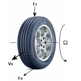
Roll and Slip
A nonslipping tire would roll and translate as Vx=rwΩ. However, as tires do slip, they respond by developing a longitudinal force, Fx.
The wheel slip velocity is Vsx=rwΩ−Vx. The wheel slip is k=VsxVx. For a locked, sliding wheel, k=−1. For perfect rolling, k=0.
Slip at Low Speed
For low speeds, as defined by Vx≤Vth, the wheel slip becomes:
k=2Vsx(Vth+V2xVth)
This modification allows for a nonsingular, nonzero slip at zero wheel velocity. For example, for perfect slipping, that is, in the case of a nontranslating spinning tire, Vx=0 while k=2rwΩVth is finite.
Deformation
If the tire is modeled with compliance, it is also flexible. In this case, because the tire deforms, the tire-road contact point turns at a slightly different angular velocity, Ω′, from the wheel, Ω, and requires, instead of the wheel slip, the contact point or contact patch slip κ'. The block models the deforming tire as a translational spring-damper of stiffness, CFx, and damping, bFx.
If you model a tire without compliance, that is, if u=0, then there is no tire longitudinal deformation at any time in the simulation and:
-
k′=k
-
V′sx=Vsx
-
Ω′=Ω
Tire and Wheel Dynamics
The full tire model is equivalent to this Simscape™/Simscape Driveline™ component diagram. It simulates both transient and steady-state behavior and correctly represents starting from, and coming to, a stop. The Translational Spring and Translational Damper are equivalent to the tire stiffness CFx and damping bFx. The Tire-Road Interaction (Magic Formula) block models the longitudinal force Fx on the tire as a function of Fz and k′ using the Magic Formula, with k′ as the independent slip variable.
The Wheel and Axle radius is the wheel radius rw. The Mass value is the effective mass, Iwr2w. The tire characteristic function f(k′, Fz) determines the longitudinal force Fx. Together with the driveshaft torque applied to the wheel axis,Fx determines the wheel angular motion and longitudinal motion.
Without tire compliance, the Translational Spring and Translational Damper are omitted, and contact variables revert to wheel variables. In this case, the tire effectively has infinite stiffness, and port P of Wheel and Axle connects directly to port T of Tire-Road Interaction (Magic Formula).
Without tire inertia, the Mass is omitted.
Assumptions and Limitations
-
The Tire (Magic Formula) block assumes longitudinal motion only and includes no camber, turning, or lateral motion.
-
Tire compliance implies a time lag in the tire response to the forces on it. Time lag simulation increases model fidelity but reduces simulation performance.
Ports
Input
N — Normal force
physical signal
Physical signal input port associated with the normal force acting on the tire. The normal force is positive if it acts downward on the tire, pressing it against the pavement.
M — Magic formula coefficients
physical signal | vector | [B, C, D, E]
Physical signal input port associated with the Magic Formula coefficients. Provide the Magic Formula coefficients as a four-element vector, specified in the order [B, C, D, E].
Dependencies
Port M is exposed only if the Main > Parameterize by parameter is set to Physical signal Magic Formula coefficients.
Output
S — Slip
physical signal
Physical signal output port associated with the relative slip between the tire and road.
Conserving
A — Axle
mechanical rotational
Mechanical rotational port associated with the axle that the tire sits on.
H — Hub
mechanical translational
Mechanical translational port associated with the wheel hub that transmits the thrust generated by the tire to the remainder of the vehicle.
Parameters
Main
The table shows how the visibility of some Main parameters depends on the options that you choose for other parameters. To learn how to read the table, see Parameter Dependencies.
Main Parameter Dependencies
| Main | |||
|---|---|---|---|
|
Parameterize by — Choose |
|||
| Peak longitudinal force and corresponding slip | Constant Magic Formula coefficients | Load-dependent Magic Formula coefficients | Physical signal Magic Formula coefficients — Exposes physical signal input port M for providing the Magic Formula coefficients to the block as an array of elements in this order [B, C, D, E]. |
|
Rated vertical load |
Magic Formula B coefficient |
Magic Formula C-coefficient parameter, p_Cx1 |
|
|
Peak longitudinal force at rated load |
Magic Formula C coefficient |
Magic Formula D-coefficient parameters, [p_Dx1 p_Dx2] |
|
|
Slip at peak force at rated load (percent) |
Magic Formula D coefficient |
Magic Formula E-coefficient parameters, [p_Ex1 p_Ex2 p_Ex3 p_Ex4] |
|
|
Magic Formula E coefficient |
Magic Formula BCD-coefficient parameters, [p_Kx1 p_Kx2 p_Kx3] |
||
|
Magic Formula H-coefficient parameters, [p_Hx1 p_Hx2] |
|||
|
Magic Formula V-coefficient parameters, [p_Vx1 p_Vx2] |
|||
Parameterize by — Parameterization method
Peak longitudinal force and corresponding slip (default) | Constant Magic Formula coefficients | Load-dependent Magic Formula coefficients | Physical signal Magic Formula coefficients
Magic Formula tire-road interaction model.
To model tire dynamics under constant pavement conditions, select one of these models:
-
Peak longitudinal force and corresponding slip— Parameterize the Magic Formula with physical characteristics of the tire. -
Constant Magic Formula coefficients— Specify the parameters that define the constant B, C, D, and E coefficients as scalars, with these default values.Coefficient Default Value B 10C 1.9D 1E 0.97 -
Load-dependent Magic Formula coefficients— Specify the parameters that define the load-dependent C, D, E, K, H, and V coefficients as vectors, one for each coefficient, with these default values.Coefficient Parameters Default Values C p_Cx1 1.685 D [ p_Dx1 p_Dx2 ] [ 1.21 –0.037 ] E [ p_Ex1 p_Ex2 p_Ex3 p_Ex4 ] [ 0.344 0.095 –0.02 0 ] K [ p_Kx1 p_Kx2 p_Kx3 ] [ 21.51 –0.163 0.245 ] H [ p_Hx1 p_Hx2 ] [ –0.002 0.002 ] V [ p_Vx1 p_Vx2 ] [ 0 0 ]
To model tire dynamics under variable pavement conditions, select Physical signal Magic Formula coefficients. Selecting this model exposes a physical signal port M. Use the port to input the Magic Formula coefficients as a four-element vector, specified in the order [B, C, D,E].
Dependencies
Each parameterization method option exposes related parameters and hides unrelated parameters. Selecting Physical signal Magic Formula coefficients exposes a physical signal input port.
Rated vertical load — Rated load force
3000 N (default) | positive scalar
Rated vertical load force Fz0.
Dependencies
This parameter is exposed only when you select the Peak longitudinal force and corresponding slip parameterization method.
Peak longitudinal force at rated load — Maximum longitudinal force at rated load
3500 N (default) | positive scalar
Maximum longitudinal force Fx0 that the tire exerts on the wheel when the vertical load equals its rated value Fz0.
Dependencies
This parameter is exposed only when you select the Peak longitudinal force and corresponding slip parameterization method. For more information, see Main Parameter Dependencies.
Slip at peak force at rated load (percent) — Percent slip at maximum longitudinal force and rated load
10 (default) | positive scalar
Contact slip κ'0, expressed as a percentage (%), when the longitudinal force equals its maximum value Fx0 and the vertical load equals its rated value Fz0.
Dependencies
This parameter is exposed only when you select the Peak longitudinal force and corresponding slip parameterization method. For more information, see Main Parameter Dependencies.
Magic Formula B coefficient — Constant Magic Formula B coefficient
10 (default) | positive scalar
Magic Formula C coefficient — Constant Magic Formula C coefficient
1.9 (default) | positive scalar
Magic Formula D coefficient — Constant Magic Formula D coefficient
1 (default) | positive scalar
Load-independent Magic Formula D coefficient.
Dependencies
This parameter is exposed only when you select the Constant Magic Formula coefficients parameterization method.
Magic Formula E coefficient — Constant Magic Formula E coefficient
0.97 (default) | positive scalar
Load-independent Magic Formula E coefficient.
Dependencies
This parameter is exposed only when you select the Constant Magic Formula coefficients parameterization method.
Tire nominal vertical load — Normal force
4000 N (default) | positive scalar
Nominal normal force Fz0 on tire.
Dependencies
This parameter is exposed only when you select the Load-dependent Magic Formula coefficients parameterization method.
Magic Formula C-coefficient parameter, p_Cx1 — Variable Magic Formula C coefficient
1.685 (default) | scalar
Load-dependent Magic Formula C coefficient.
Dependencies
This parameter is exposed only when you select the Load-dependent Magic Formula coefficients parameterization method.
Magic Formula D-coefficient parameters, [p_Dx1 p_Dx2] — Variable Magic Formula D coefficient
[1.21, -.037] (default) | vector
Load-dependent Magic Formula D coefficient.
Dependencies
This parameter is exposed only when you select the Load-dependent Magic Formula coefficients parameterization method.
Magic Formula E-coefficient parameters, [p_Ex1 p_Ex2 p_Ex3 p_Ex4] — Variable Magic Formula E coefficient
[.344, .095, -.02, 0] (default) | vector
Load-dependent Magic Formula E coefficient.
Dependencies
This parameter is exposed only when you select the Load-dependent Magic Formula coefficients parameterization method Magic Formula BCD-coefficient parameters, [p_Kx1 p_Kx2 p_Kx3] — Variable Magic Formula K coefficient[21.51, -.163, .245] (default) | vector
Load-dependent Magic Formula K coefficient.
Dependencies
This parameter is exposed only when you select the Load-dependent Magic Formula coefficients parameterization method.
Magic Formula H-coefficient parameters, [p_Hx1 p_Hx2] — Variable Magic Formula H coefficient
[-.002, .002] (default) | vector
Load-dependent Magic Formula H coefficient.
Dependencies
This parameter is exposed only when you select the Load-dependent Magic Formula coefficients parameterization method.
Magic Formula V-coefficient parameters, [p_Vx1 p_Vx2] — Variable Magic Formula V coefficient
[0, 0] (default) | vector
Load-dependent Magic Formula V coefficient.
Dependencies
This parameter is exposed only when you select the Load-dependent Magic Formula coefficients parameterization method.
Geometry
Rolling radius — Unloaded tire-wheel radius
0.3 m (default) | positive scalar
Unloaded tire-wheel radius, rw.
Dynamics
The table shows how the visibility of some Dynamics parameters depends on the options that you choose for other parameters. .
Dynamics Parameter Dependencies
| Dynamics | |
|---|---|
|
Compliance — Choose |
|
| No compliance - Suitable for HIL simulation | Specify stiffness and damping |
|
Longitudinal stiffness |
|
|
Longitudinal damping |
|
|
Inertia — Choose |
|
| No Inertia | Specify inertia and initial velocity |
|
Tire inertia |
|
|
Initial velocity |
|
Compliance — Dynamical compliance model
No compliance - Suitable for HIL simulation (default) | Specify stiffness and damping
Model for the dynamical compliance of the tire.
-
No compliance - Suitable for HIL simulation— Tire is modeled with no dynamical compliance. -
Specify stiffness and damping— Tire is modeled as a stiff, dampened spring and deforms under load.
Dependencies
Selecting the Specify stiffness and damping parameterization method, exposes stiffness and damping parameters.
Longitudinal stiffness — Longitudinal stiffness
1e6 N/m (default) | positive scalar
Tire longitudinal stiffness CFx.
Dependencies
Selecting Specify stiffness and damping for the Compliance parameter, exposes this parameter.
Longitudinal damping — Longitudinal damping
1000 N/(m/s) (default) | positive scalar
Tire longitudinal damping bFx.
Dependencies
Selecting Specify stiffness and damping for the Compliance parameter, exposes this parameter.
Inertia — Inertia model
No inertia (default) | Specify inertia and initial velocity
Model for the rotational inertia of the tire.
-
No inertia— Tire is modeled with no dynamical compliance. -
Specify inertia and initial velocity— Tire is modeled as a stiff, dampened spring and deforms under load.
Dependencies
Selecting the Specify inertia and initial velocity parameterization method, exposes inertia and velocity parameters. For more information, see Dynamics Parameter Dependencies.
Tire inertia — Rotational inertia
1 kg*m^2 (default) | positive scalar
Rotational inertia Iw of the wheel-tire assembly.
Dependencies
Selecting Specify inertia and initial velocity for the Inertia parameter, exposes this parameter. Initial velocity — Initial rotational velocity0 rad/s (default) | scalar
Initial angular velocity, Ω(0), of the tire.
Dependencies
Selecting Specify inertia and initial velocity for the Inertia parameter, exposes this parameter. Rolling Resistance
The table shows how the visibility of some parameters depends on the options that you choose for other parameters.
Rolling Resistance Parameter Dependencies
| Rolling Resistance | ||
|---|---|---|
|
Rolling resistance — Choose |
||
| Off | On | |
|
Resistance model — Choose |
||
| Constant coefficient | Pressure and velocity dependent | |
|
Constant coefficient |
Tire pressure |
|
|
Alpha |
||
|
Beta |
||
|
Coefficient A |
||
|
Coefficient B |
||
|
Coefficient C |
||
|
Velocity threshold |
||
Rolling resistance — Rolling resistance option
Off (default) | On
Options for modeling rolling resistance are:
-
Off— Neglect rolling resistance. -
On— Include rolling resistance.
Dependencies
Selecting On exposes rolling resistance parameters.
Resistance model — Rolling resistance model
Constant coefficient (default) | Pressure and velocity dependent
Model for the rolling resistance of the tire.
-
Constant coefficient— Neglect rolling resistance. -
Pressure and velocity dependent— Include rolling resistance.
Dependencies
Each Resistance model option exposes related parameters. For more information, see Rolling Resistance Parameter Dependencies.
Constant coefficient — Proportionality constant
0.015 (default) | positive scalar
Coefficient that sets the proportionality between the normal force and the rolling resistance force. The parameter must be greater than zero.
Dependencies
Selecting On for the Rolling resistance parameter and Constant coefficient for the Resistance model parameter exposes this parameter.
Tire pressure — Tire pressure
250e3 Pa (default) | positive scalar
Inflation pressure of the tire. The parameter must be greater than zero.
Dependencies
Selecting On for the Rolling resistance parameter and Pressure and velocity dependent for the Resistance model parameter exposes this parameter.
Alpha — Tire pressure equation exponent
-0.003 (default) | scalar
Exponent of the tire pressure in the model equation.
Dependencies
Selecting On for the Rolling resistance parameter and Pressure and velocity dependent for the Resistance model parameter exposes this parameter.
Beta — Normal force equation exponent
0.97 (default) | scalar
Exponent of the normal force model equation.
Dependencies
Selecting On for the Rolling resistance parameter and Pressure and velocity dependent for the Resistance model parameter exposes this parameter.
Coefficient A — Velocity-independent force component A
84e-4 (default)
Velocity-independent force component in the model equation. The parameter must be greater than zero.
Dependencies
Selecting On for the Rolling resistance parameter and Pressure and velocity dependent for the Resistance model parameter exposes this parameter.
Coefficient B — Velocity-dependent force component B
6.2e-4 s/m (default) | positive scalar
Velocity-dependent force component in the model equation. The parameter must be greater than zero.
Dependencies
Selecting On for the Rolling resistance parameter and Pressure and velocity dependent for the Resistance model parameter exposes this parameter.
Coefficient C — Velocity-dependent force component C
1.6e-4 s^2/m^2 (default) | positive scalar
Force component that depends on the square of the velocity term in the model equation. The parameter must be greater than zero.
Dependencies
Selecting On for the Rolling resistance parameter and Pressure and velocity dependent for the Resistance model parameter exposes this parameter.
Velocity threshold — Wheel hub velocity threshold for mathematical slip model
0.001 m/s (default) | positive scalar
Velocity at which the full rolling resistance force is transmitted to the rolling hub. The parameter ensures that the force remains continuous during velocity direction changes, which increases the numerical stability of the simulation. The parameter must be greater than zero.
Dependencies
Selecting On for the Rolling resistance parameter exposes this parameter.
Advanced
Velocity threshold — Wheel hub velocity threshold for mathematical slip model
0.1 m/s (default) | positive scalar
Wheel hub velocity Vth below which the slip calculation is modified to avoid singular evolution at zero velocity. Must be positive.
PS Terminator
Terminator for unconnected physical signal outputs
Library
Physical Signals/Sinks
Description
Use the PS Terminator block to cap physical signal output ports that do not connect to other blocks.
Unlike conserving ports in physical modeling, or Simulink® output ports, unconnected physical signal output ports do not generate warnings. However, you can use a PS Terminator block for clarity, to indicate that the signal was not inadvertently left unconnected.
The block icon size allows you to connect the PS Terminator block to an open port without rerouting the adjacent lines:
Ports
The block has one physical signal input port.
Double-Shoe Brake
Frictional brake with two pivoted shoes diametrically positioned about a rotating drum
Library
Brakes & Detents/Rotational
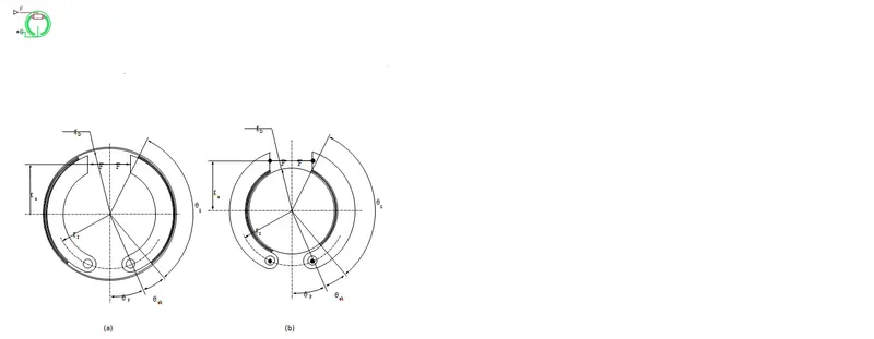
Description
The block represents a frictional brake with two pivoted rigid shoes that press against a rotating drum to produce a braking action. The rigid shoes sit inside or outside the rotating drum in a diametrically opposed configuration. A positive actuating force causes the rigid shoes to press against the rotating drum. Viscous and contact friction between the drum and the rigid shoe surfaces cause the rotating drum to decelerate. Double-shoe brakes provide high braking torque with small actuator deflections in applications that include motor vehicles and some heavy machinery. The model employs a simple parameterization with readily accessible brake geometry and friction parameters.
In this schematic, a) represents an internal double-shoe brake, and b) represents an external double-shoe brake. In both configurations, a positive actuation force F brings the shoe and drum friction surfaces into contact. The result is a friction torque that causes deceleration of the rotating drum. Zero and negative forces do not bring the shoe and drum friction surfaces into contact and produce zero braking torque.
The model uses the long-shoe approximation. Contact angles smaller than 45° produce less accurate results. The equations for the friction torque that the leading and trailing shoes develop are:
TLS=cμparD2(cosθsb−cosθs)sinθa,
TTS=cμpbrD2(cosθsb−cosθs)sinθa,
c=ra+rpcosθp,
where for 0≤θs≤π/2,
θa=θs,
and for θs≥π/2,
θa=π2.
The parameters in the friction torque equations are:
| Parameter | Description |
|---|---|
| TLS | Brake torque the leading shoe develops |
| TTS | Brake torque the trailing shoe develops |
| μ | Effective contact friction coefficient |
| pa | Maximum linear pressure in the leading shoe-drum contact |
| pb | Maximum linear pressure in the trailing shoe-drum contact |
| rD | Drum radius |
| θsb | Shoe beginning angle |
| θs | Shoe span angle |
| θa | Angle from hinge pin to maximum pressure point |
| c | Arm length of the cylinder force with respect to the hinge pin |
| rp | Pin location radius |
| θp | Hinge pin location angle |
| ra | Actuator location radius |
The model assumes that only Coulomb friction acts at the shoe-drum surface contact. Zero relative velocity between the drum and the shoes produces zero Coulomb friction. To avoid discontinuity at zero relative velocity, the friction coefficient formula employs this hyperbolic function
μ=μCoulombtanh(4ωshaftωthreshold),
where:
| Parameter | Description |
|---|---|
| μ | Effective contact friction coefficient |
| μCoulomb | Contact friction coefficient |
| ωshaft | Shaft velocity |
| ωthreshold | Angular velocity threshold |
Balancing the moments that act on each shoe with respect to the pin yields the pressure acting at the shoe-drum surface contact. The equations for determining the balance of moments for the leading shoe are
F=MN−MFc,
MN=parprDsinθa(12[θs−θsb]−14[sin2θs−sin2θsb]),
and
MF=μparDsinθa(rD[cosθsb−cosθs]+rp4[cos2θs−cos2θsb]),
where:
| Parameter | Description |
|---|---|
| F | Actuation Force |
| MN | Moment acting on the leading shoe due to normal force |
| MF | Moment acting on the leading shoe due to friction force |
| c | Arm length of the cylinder force with respect to the hinge pin |
| pa | Maximum linear pressure at the shoe-drum contact surface |
| rp | Pin location radius |
| θp | Hinge pin location angle |
| ra | Actuator location radius |
The model does not simulate self-locking brakes. If brake geometry and friction parameters cause a self-locking condition, the model produces a simulation error. A brake self-locks if the friction moment exceeds the moment due to normal forces, that is, when MF > MN.
The balance of moments for the trailing shoe is
F=MN+MFc.
The net braking torque is
T=TLS+TTS+μvisc∗ωshaft,
where μvisc is the viscous friction coefficient.
Variables
Use the Variables tab to set the priority and initial target values for the block variables before simulating.
Unlike block parameters, variables do not have conditional visibility. The Variables tab lists all the existing block variables. If a variable is not used in the set of equations corresponding to the selected block configuration, the values specified for this variable are ignored.
Assumptions and Limitations
-
The brake uses the long-shoe approximation.
-
The brake geometry does not self-lock.
-
The model does not account for actuator flow consumption.
Thermal Modeling
You can model the effects of heat flow and temperature change through an optional thermal conserving port. By default, the thermal port is hidden. To expose the thermal port, right-click the block in your model and, from the context menu, select Simscape > Block choices. Select a variant that includes a thermal port. Specify the associated thermal parameters for the component.
Ports
F-
Physical signal port that represents the brake actuating force
S-
Rotational conserving port that represents the rotating drum shaft
H-
Thermal conserving port. The thermal port is optional and is hidden by default. To expose the port, select a variant that includes a thermal port.
Parameters
Geometry
- Drum radius
-
Radius of the drum contact surface. The parameter must be greater than zero. The default value is
150mm. - Actuator location radius
-
Distance between the drum center and the force line of action. The parameter must be greater than zero. The default value is
100mm. - Pin location radius
-
Distance between the hinge pin and drum centers. The parameter must be greater than zero. The default value is
125mm. - Pin location angle
-
Angular coordinate of the hinge pin location from the brake symmetry axis. The parameter must be greater than or equal to zero. The default value is
15deg. - Shoe beginning angle
-
Angle between the hinge pin and the beginning of the friction material linen of the shoe. The value of the parameter must be in the range 0 ≤ θsb ≤ (π-pin location angle). The default value is
5deg. - Shoe span angle
-
Angle between the beginning and the end of the friction material linen on the shoe. The value of the parameter must be in the range 0 < θsb ≤ (π -pin location angle - shoe beginning angle). The default value is
120deg.
Friction
- Viscous friction coefficient
-
Value of the viscous friction coefficient at the contact surface. The parameter must be greater than or equal to zero. The default value is
.01n*m/(rad/s). - Temperature
-
Array of temperatures used to construct a 1-D temperature-efficiency lookup table. The array values must increase left to right. The default value is
[280.0, 300.0, 320.0]K.This parameter is visible only when you select a block variant that includes a thermal port.
- Contact friction coefficient
-
Value of the Coulomb friction coefficient at the belt-drum contact surface. The value is greater than zero. Unless you select a block variant that includes a thermal port, the default value is
0.3.If you select a block variant that includes a thermal port, you specify this parameter as array. The array is the same size as the array for the Temperature parameter. The default value for the thermal variant is
[0.1, 0.05, 0.03]. - Angular velocity threshold
-
Angular velocity at which the contact friction coefficient practically reaches its steady-state value. The parameter must be greater than zero. The default value is
0.01rad/s.
Thermal Port
- Thermal mass
-
Thermal energy required to change the component temperature by a single degree. The greater the thermal mass, the more resistant the component is to temperature change. This parameter is enabled only if you select a block variant that includes a thermal port. The default value is
50kJ/K.
Vehicle Body
Two-axle vehicle with longitudinal dynamics and motion and adjustable mass, geometry, and drag properties
- Library:
-
Simscape / Driveline / Tires & Vehicles
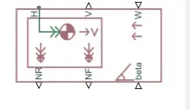
Description
The Vehicle Body block represents a two-axle vehicle body in longitudinal motion. The vehicle can have the same or a different number of wheels on each axle. For example, two wheels on the front axle and one wheel on the rear axle. The vehicle wheels are assumed identical in size. The vehicle can also have a center of gravity (CG) that is at or below the plane of travel.
The block accounts for body mass, aerodynamic drag, road incline, and weight distribution between axles due to acceleration and road profile. Optionally include pitch and suspension dynamics. The vehicle does not move vertically relative to the ground.
Model
The vehicle axles are parallel and form a plane. The longitudinal, x, direction lies in this plane and perpendicular to the axles. If the vehicle is traveling on an incline slope, β, the normal, z, direction is not parallel to gravity but is always perpendicular to the axle-longitudinal plane.
This figure and table define the vehicle motion model variables.
Vehicle Dynamics and Motion
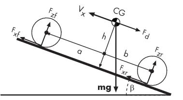
Vehicle Model Variables
| Symbol | Description |
|---|---|
| g | Gravitational acceleration |
| β | Incline angle |
| m | Mass of the vehicle |
| h | Height of vehicle center of gravity (CG) above the ground |
| a, b | Distance of front and rear axles, respectively, from the normal projection point of vehicle CG onto the common axle plane |
| Vx | Velocity of the vehicle. When Vx > 0, the vehicle moves forward. When Vx < 0, the vehicle moves backward. |
| Vw | Wind speed. When Vw > 0, the wind is headwind. When Vw < 0, the wind is tailwind. |
| n | Number of wheels on each axle |
| Fxf, Fxr | Longitudinal forces on each wheel at the front and rear ground contact points, respectively |
| Fzf, Fzr | Normal load forces on each wheel at the front and rear ground contact points, respectively |
| A | Effective frontal vehicle cross-sectional area |
| Cd | Aerodynamic drag coefficient |
| ρ | Mass density of air |
| Fd | Aerodynamic drag force |
Equations
Vehicle Dynamics
The vehicle motion is a result of the net effect of all the forces and torques acting on it. The longitudinal tire forces push the vehicle forward or backward. The weight mg of the vehicle acts through its center of gravity (CG). Depending on the incline angle, the weight pulls the vehicle to the ground and pulls it either backward or forward. Whether the vehicle travels forward or backward, aerodynamic drag slows it down. For simplicity, the drag is assumed to act through the CG.
m˙Vx=Fx− Fd−mg⋅sinβ
Fx=n(Fxf+Fxr)
Fd=12CdρA(Vx+Vw)2⋅sgn(Vx+Vw)
Zero normal acceleration and zero pitch torque determine the normal force on each front and rear wheel.
Fzf=−h(Fd+mgsinβ+m˙Vx)+b⋅mgcosβn(a+b)
Fzr=+h(Fd+mgsinβ+m˙Vx)+a⋅mgcosβn(a+b)
The wheel normal forces satisfy Fzf+Fzr=mgcosβn.
Pitch dynamics
The rate of the pitch that occurs during vehicle acceleration depends on three torque components and the inertia of the vehicle:
α=(f⋅h)+(Fzfa)−(Fzrb)J
Where:
-
ɑ is the pitch rate.
-
f is the longitudinal force.
-
J is the inertia.
If you choose a linear model for suspension stiffness and damping, the block uses small angle approximation for pitch calculations. If you choose a table lookup model, the block uses the vectors that you specify calculate pitch dynamics.
Variables
Use the Variables tab to set the priority and initial target values for the block variables before simulating. For more information, see Set Priority and Initial Target for Block Variables (Simscape).
Unlike block parameters, variables do not have conditional visibility. The Variables tab lists all the existing block variables. If a variable is not used in the set of equations corresponding to the selected block configuration, the values specified for this variable are ignored.
Limitations and Assumptions
The Vehicle Body block lets you model only longitudinal dynamics, parallel to the ground and oriented along the direction of motion. The vehicle is assumed to be in pitch and normal equilibrium. The block does not model pitch or vertical movement. As such, the equations assume that the wheels never lose contact. This constraint can result in negative normal forces.
Ports
Input
W — Headwind speed
scalar
Physical signal input port for headwind speed.
beta — Road incline angle
scalar
Physical signal input port for road incline angle.
Output
V — Longitudinal velocity
scalar
Physical signal output port for vehicle longitudinal velocity.
NF — Front axle normal force
scalar
Physical signal output port for normal force on the front axle. Wheel forces are considered positive if acting downwards.
NR — Rear axle normal force
scalar
Physical signal output port for normal force on the rear axle. Wheel forces are considered positive if acting downwards.
Conserving
H — Horizontal motion
mechanical translational
Conserving port associated with the horizontal motion of the vehicle body. Connect tire traction motion to this port.
Parameters
Main
Mass — Vehicle mass
1200 kg (default)
Mass of the vehicle.
Number of wheels per axle — Wheel count
2 (default) | scalar number or a two-element array
Wheel counts on the front and rear axles. If the input is a scalar number, the wheel counts of the front and rear axles are assumed the same. For example, if the input is 2, then the front and rear axles are each assumed to have two wheels.
If the input is a two-element array, the first number is the front-axle wheel count and the second number the rear-axle wheel count. For example, if the input is the array [2,1], then the front axle is assumed to have two wheels and the rear axle one wheel.
Horizontal distance from CG to front axle — CG-to-front axle distance
1.4 m (default)
Horizontal distance, a, from the center of gravity to the front wheel axle of the vehicle.
Horizontal distance from CG to rear axle — CG-to-rear axle distance
1.6 m (default)
Horizontal distance, b, from the center of gravity to the rear wheel axle of the vehicle.
CG height above ground — CG-to-ground distance
0.5 m (default)
Distance, h, between the center of gravity of the vehicle and the ground.
Gravitational acceleration — Gravitational acceleration
9.81 m/s^2 (default)
Acceleration due to gravitational force acting at the center of gravity of the vehicle.
Negative normal force warning — Warning
Off (default) | On
To see a warning when the block calculates negative values for normal force during simulation, select On. The block can generate negative forces because the equations assume that the wheels never lose contact.
Drag
Frontal area — Effective cross-sectional area
3 m^2 (default)
Effective cross-sectional area, A, presented by the vehicle in longitudinal motion. The block uses this value to calculate the aerodynamic drag force on the vehicle.
Drag coefficient — Aerodynamic drag coefficient
0.4 (default)
Aerodynamic drag coefficient, Cd. The block uses this value to calculate the aerodynamic drag force on the vehicle.
Air density — Ambient air density
1.18 kg/m^3 (default)
Density of the air that surrounds the vehicle.
Pitch
The table shows how the visibility of some parameters depends on the option that you choose for other parameters.
Pitch Parameter Dependencies
| Pitch | ||
|---|---|---|
Pitch dynamics — Choose Off or On |
||
| Off | On | |
| Pitch moment of inertia | ||
Suspension model — Choose Linear or By table lookup |
||
| Linear | By table lookup | |
| Front suspension stiffness | Front suspension stiffness force vector | |
| Front suspension damping | Front suspension deformation vector | |
| Rear suspension stiffness | Front suspension damping force vector | |
| Rear suspension damping | Front suspension velocity vector | |
| Rear suspension stiffness force vector | ||
| Rear suspension deformation vector | ||
| Rear suspension damping force vector | ||
| Rear suspension velocity vector | ||
| Interpolation method | ||
| Extrapolation method | ||
Hard stop — Choose Off or On |
||
| Off | On | |
| Front upper bound | ||
| Front lower bound | ||
| Front contact stiffness | ||
| Front contact damping | ||
| Rear upper bound | ||
| Rear lower bound | ||
| Rear contact stiffness | ||
| Rear contact damping | ||
| Initial pitch | ||
| Initial pitch rate | ||
Pitch dynamics — Pitch dynamics modelling
Off (default) | On
Option to model pitch dynamics.
Dependencies
Selecting On for this parameter enables parameters for:
-
Suspension model
-
Hard-stop model
-
Initial pitch conditions
Pitch moment of inertia — Pitch moment of inertia
4000 kg/m^2 (default) | positive scalar
Moment of inertia for pitch calculations.
Dependencies
This parameter is enabled when you set Pitch dynamics to On.
Suspension model — Suspension parameterization method
Linear (default) | Table lookup
Parameterization method for suspension modeling.
You parameterize the suspension using stiffness and damping data. To specify the data using scalar values, select Linear. To specify the data using vector values, select By table lookup.
Dependencies
This parameter is enabled when you set Pitch dynamics to On.
Front suspension stiffness — Front suspension stiffness
1e4 N/m (default) | positive scalar
Front suspension stiffness per axle.
Dependencies
This parameter is enabled when you set both of these options:
-
Pitch dynamics to
On -
Suspension model to
Linear
Front suspension damping — Front suspension damping
1e4N/(m/s) (default) | positive scalar
Front suspension damping per axle.
Dependencies
This parameter is enabled when you set both of these options:
-
Pitch dynamics to
On -
Suspension model to
Linear
Rear suspension stiffness — Rear suspension stiffness
1e4 N/m (default) | positive scalar
Rear suspension stiffness per axle.
Dependencies
This parameter is enabled when you set both of these options:
-
Pitch dynamics to
On -
Suspension model to
Linear
Rear suspension damping — Rear suspension damping
1e4N/(m/s) (default) | positive scalar
Rear suspension damping per axle.
Dependencies
This parameter is enabled when you set both of these options:
-
Pitch dynamics to
On -
Suspension model to
Linear
Front suspension stiffness force vector — Front suspension stiffness force
[-2000, -1000, 0, 1000, 2000] N (default) | increasing vector
Stiffness force of the front suspension. Specify the output values for the lookup table as a vector. The number of elements in the output vector must be the same as the number of elements in the input vector. The input vector parameter is the Front suspension deformation vector parameter.
Dependencies
This parameter is enabled when you set both of these options:
-
Pitch dynamics to
On -
Suspension model to
By table lookup
Front suspension deformation vector — Front suspension deformation
[-.4, -.2, 0, .2, .4] m (default) | increasing vector
Deformation of the front suspension specified in terms of displacement. Specify the input values for the lookup table as a vector. The values of the elements in the vector must increase from left to right. The minimum number of elements in the vector depends on the interpolation method that you select. For linear interpolation, provide at least two elements. For smooth interpolation, provide at least three elements. The output vector parameter is the Front suspension stiffness force vector parameter.
Dependencies
This parameter is enabled when you set both of these options:
-
Pitch dynamics to
On -
Suspension model to
By table lookup
Front suspension damping force vector — Front suspension damping force
[-200, -100, 0, 100, 200] N (default) | increasing vector
Damping force of the front suspension. Specify the output values for the lookup table as a vector. The number of elements in the output vector must be the same as the number of elements in the input vector. The input vector parameter is the Front suspension velocity vector parameter.
Dependencies
This parameter is enabled when you set both of these options:
-
Pitch dynamics to
On -
Suspension model to
By table lookup
Front suspension velocity vector — Front suspension velocity
[-4, -2, 0, 2, 4] m/s (default) | increasing vector
Velocity of the front suspension. Specify the input values for the lookup table as a vector. The values of the elements in the vector must increase from left to right. The minimum number of elements in the vector depends on the interpolation method that you select. For linear interpolation, provide at least two elements. For smooth interpolation, provide at least three elements. The output vector parameter is the Front suspension damping force vector parameter.
Dependencies
This parameter is enabled when you set both of these options:
-
Pitch dynamics to
On -
Suspension model to
By table lookup
Rear suspension stiffness force vector — Rear suspension stiffness force
[-2000, -1000, 0, 1000, 2000] N (default) | increasing vector
Stiffness force of the rear suspension. Specify the output values for the lookup table as a vector. The number of elements in the output vector must be the same as the number of elements in the input vector. The input vector parameter is the Rear suspension deformation vector parameter.
Dependencies
This parameter is enabled when you set both of these options:
-
Pitch dynamics to
On -
Suspension model to
By table lookup
For more information, see the Pitch Parameter Dependencies table.
Rear suspension deformation vector — Rear suspension deformation
[-.4, -.2, 0, .2, .4] m (default) | increasing vector
Deformation of the rear suspension specified in terms of displacement. Specify the input values for the lookup table as a vector. The values of the elements in the vector must increase from left to right. The minimum number of elements in the vector depends on the interpolation method that you select. For linear interpolation, provide at least two elements. For smooth interpolation, provide at least three elements. The output vector parameter is the Rear suspension stiffness force vector parameter.
Dependencies
This parameter is enabled when you set both of these options:
-
Pitch dynamics to
On -
Suspension model to
By table lookup
Rear suspension damping force vector — Rear suspension damping force
[-200, -100, 0, 100, 200] N (default) | increasing vector
Damping force of the rear suspension. Specify the output values for the lookup table as a vector. The number of elements in the output vector must be the same as the number of elements in the input vector. The input vector parameter is the Rear suspension velocity vector parameter.
Dependencies
This parameter is enabled when you set both of these options:
-
Pitch dynamics to
On -
Suspension model to
By table lookup
Rear suspension velocity vector — Rear suspension velocity
[-4, -2, 0, 2, 4] m/s (default) | increasing vector
Velocity of the rear suspension. Specify the input values for the lookup table as a vector. The values of the elements in the vector must increase from left to right. The minimum number of elements in the vector depends on the interpolation method that you select. For linear interpolation, provide at least two elements. For smooth interpolation, provide at least three elements. The output vector parameter is the Rear suspension damping force vector parameter.
Dependencies
This parameter is enabled when you set both of these options:
-
Pitch dynamics to
On -
Suspension model to
By table lookup
Interpolation method — Interpolation method
linear (default) | smooth
Interpolation methods for approximating the output value when the input value is between two consecutive grid points are:
-
Linear— Select this default option to get the best performance. Provide at least two values per dimension. -
Smooth— Select this option to produce a continuous curve with continuous first-order derivatives. Provide at least three values per dimension.
Dependencies
This parameter is enabled when you set both of these options:
-
Pitch dynamics to
On -
Suspension model to
By table lookup
Extrapolation method — Extrapolation method
linear (default) | smooth
Extrapolation method for determining the output value when the input value is outside the range specified in the argument list are:
-
Linear— Produces a curve with continuous first-order derivatives in the extrapolation region and at the boundary with the interpolation region. -
Nearest— Produces an extrapolation that does not go above the highest point in the data or below the lowest point in the data.
Dependencies
This parameter is enabled when you set both of these options:
-
Pitch dynamics to
On -
Suspension model to
By table lookup
Hard stop — Hard-stop modeling option
Off (default) | On
Option to model hardstops for the front and rear suspension.
Dependencies
This parameter is enabled when you set the Pitch dynamics to On:
Selecting On for this parameter enables parameters for the front and rear hard stops:
-
Upper bound
-
Lower bound
-
Contact stiffness
-
Contact damping
Front upper bound — Hardstop front suspension upper bound
.25 (default)
Upper bound of the hard stop for the front suspension.
Dependencies
This parameter is enabled when you set both of these options:
-
Pitch dynamics to
On -
Hard stop to
On
For more information, see the Pitch Parameter Dependencies table.
Front lower bound — Vehicle front lower bound
-.25 (default)
Front contact stiffness — Vehicle front contact stiffness
1e6 (default)
Front contact damping — Vehicle front contact damping
150 (default)
Rear upper bound — Vehicle rear upper bound
.25 (default)
Upper bound of the hard stop for the rear suspension.
Dependencies
This parameter is enabled when you set both of these options:
-
Pitch dynamics to
On -
Hard stop to
On
Rear lower bound — Vehicle rear lower bound
-.25 (default)
Lower bound of the hard stop for the rear suspension.
Dependencies
This parameter is enabled when you set both of these options:
-
Pitch dynamics to
On -
Hard stop to
On
Rear contact stiffness — Vehicle rear contact stiffness
1e6 (default)
Contact stiffness of the hard stop for the rear suspension.
Dependencies
This parameter is enabled when you set both of these options:
-
Pitch dynamics to
On -
Hard stop to
On
Rear contact damping — Vehicle rear contact damping
150 (default)
Contact damping of the hard stop for the rear suspension.
Dependencies
This parameter is enabled when you set both of these options:
-
Pitch dynamics to
On -
Hard stop to
On
Initial pitch — Pitch at the beginning of the simulation
0 rad (default)
Pitch at the beginning of the simulation.
Dependencies
This parameter is enabled when you set Pitch dynamics to On.
Initial pitch rate — Pitch rate at the beginning of the simulation
0 rad/s (default)
Pitch rate at the beginning of the simulation.
Dependencies
This parameter is enabled when you set Pitch dynamics to On.
.
n-D Lookup Table
Approximate n-dimensional function
- Library:
-
Simulink / Lookup Tables
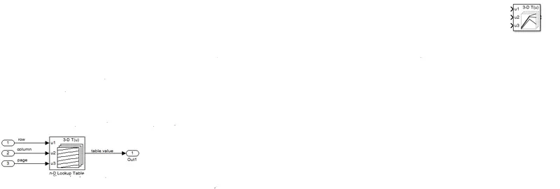
Description
Supported Block Operations
The 1-D, 2-D, and n-D Lookup Table blocks evaluate a sampled representation of a function in N variables
y=F(x1,x2,x3,...,xN)
where the function F can be empirical. The block maps inputs to an output value by looking up or interpolating a table of values you define with block parameters. The block supports flat (constant), linear (Linear point-slope), Lagrange (Linear Lagrange), nearest, and cubic-spline interpolation methods. You can apply these methods to a table of any dimension from 1 through 30.
In the following block, the first input identifies the first dimension (row) breakpoints, the second input identifies the second dimension (column) breakpoints, and so on.
See Port Location After Rotating or Flipping for a description of the port order for various block orientations.
When the Math and Data Types > Use algorithms optimized for row-major array layout configuration parameter is set, the 2-D and n-D Lookup Table block behavior changes from column-major to row-major. For these blocks, the column-major and row-major algorithms may differ in the order of the output calculations, possibly resulting in slightly different numerical values. This capability requires a Simulink® Coder™ or Embedded Coder®license. For more information on row-major support, see Code Generation of Matrices and Arrays (Simulink Coder).
Specification of Breakpoint and Table Data
These block parameters define the breakpoint and table data.
| Block Parameter | Purpose |
|---|---|
| Number of table dimensions | Specifies the number of dimensions of your lookup table. |
| Breakpoints | Specifies a breakpoint vector that corresponds to each dimension of your lookup table. |
| Table data | Defines the associated set of output values. |
Tip
Evenly spaced breakpoints can make the generated code division-free. For more information, see fixpt_evenspace_cleanup and Identify questionable fixed-point operations (Embedded Coder).
How the Block Generates Output
The n-D, 1-D and 2-D Lookup Table blocks generate output by looking up or estimating table values based on the input values.
| When block inputs... | The n-D Lookup Table block... |
|---|---|
| Match the values of indices in breakpoint data sets | Outputs the table value at the intersection of the row, column, and higher dimension breakpoints |
| Do not match the values of indices in breakpoint data sets, but are within range | Interpolates appropriate table values, using the Interpolation method you select |
| Do not match the values of indices in breakpoint data sets, and are out of range | Extrapolates the output value, using the Extrapolation method you select |
Other Blocks that Perform Equivalent Operations
You can use the Interpolation Using Prelookup block with the Prelookup block to perform the equivalent operation of one n-D Lookup Table block. This combination of blocks offers greater flexibility that can result in more efficient simulation performance for linear interpolations.
When the lookup operation is an array access that does not require interpolation, use the Direct Lookup Table (n-D) block. For example, if you have an integer value k and you want the kth element of a table, y = table(k), interpolation is unnecessary.
Ports
Input
u1 — First-dimension (row) inputs
scalar | vector | matrix
Real-valued inputs to the u1 port, mapped to an output value by looking up or interpolating the table of values that you define.
Example: 0:10
Data Types: single | double | int8 | int16 | int32 | uint8 | uint16 | uint32 | fixed point
uN — n-th dimension input values
scalar | vector | matrix
Real-valued inputs to the uN port, mapped to an output value by looking up or interpolating the table of values that you define.
Example: 0:10
Data Types: single | double | int8 | int16 | int32 | uint8 | uint16 | uint32 | fixed point
Output
Port_1 — Output computed by looking up or estimating table values
scalar | vector | matrix
Output generated by looking up or estimating table values based on the input values:
| When block inputs... | The n-D Lookup Table block... |
|---|---|
| Match the values of indices in breakpoint data sets | Outputs the table value at the intersection of the row, column, and higher dimension breakpoints |
| Do not match the values of indices in breakpoint data sets, but are within range | Interpolates appropriate table values, using the Interpolation method you select |
| Do not match the values of indices in breakpoint data sets, and are out of range | Extrapolates the output value, using the Extrapolation method you select |
Data Types: single | double | int8 | int16 | int32 | uint8 | uint16 | uint32 | fixed point
Parameters
Table and Breakpoints
Number of table dimensions — Number of lookup table dimensions
3 (default) | 1 | 2 | 4 | ... | 30
Enter the number of dimensions of the lookup table. This parameter determines:
-
The number of independent variables for the table and the number of block inputs
-
The number of breakpoint sets to specify
| To specify... | Do this... |
|---|---|
|
1, 2, 3, or 4 |
Select the value from the drop-down list. |
|
A higher number of table dimensions |
Enter a positive integer directly in the field. The maximum number of table dimensions that this block supports is 30. |
Programmatic Use
Block Parameter: NumberOfTableDimensions |
| Type: character vector |
Values: '1' | '2' | '3' | '4' | ... | 30 |
Default: '3' |
Data specification — Method of table and breakpoint specification
Table and breakpoints (default) | Lookup table object
From the list, select:
-
Table and breakpoints— Specify the table data and breakpoints. Selecting this option enables the following parameters:-
Table data
-
Breakpoints specification
-
Breakpoints 1
-
Breakpoints 2
-
Breakpoints 3
-
Edit table and breakpoints
-
-
Lookup table object— Use an existing lookup table (Simulink.LookupTable) object. Selecting this option enables the Name field and Edit table and breakpoints button.
Programmatic Use
Block Parameter: DataSpecification |
| Type: character vector |
Values: 'Table and breakpoints' | 'Lookup table object' |
Default: 'Table and breakpoints' |
Name — Name of the lookup table object
[] (default) | Simulink.LookupTable object
Enter the name of the lookup table (Simulink.LookupTable) object.
Dependencies
To enable this parameter, set Data specification to Lookup table object.
Programmatic Use
Block Parameter: LookupTableObject |
| Type: character vector |
Values: name of a Simulink.LookupTable object |
Default: '' |
Table data — Define the table of output values
reshape(repmat([4 5 6;16 19 20;10 18 23],1,2),[3,3,2]) (default) | matrix of values with dimensions that match the Number of table dimensions
Enter the table of output values.
During simulation, the matrix size must match the dimensions defined by the Number of table dimensions parameter. However, during block diagram editing, you can enter an empty matrix (specified as []) or an undefined workspace variable. This technique lets you postpone specifying a correctly dimensioned matrix for the table data and continue editing the block diagram.
Dependencies
To enable this parameter, set Data specification to Table and breakpoints.
Programmatic Use
Block Parameter: Table |
| Type: character vector |
| Values: matrix of table values |
Default: 'reshape(repmat([4 5 6;16 19 20;10 18 23],1,2),[3,3,2])' |
Breakpoints specification — Method of breakpoint specification
Explicit values (default) | Even spacing
Specify whether to enter data as explicit breakpoints or as parameters that generate evenly spaced breakpoints.
-
To explicitly specify breakpoint data, set this parameter to
Explicit valuesand enter breakpoint data in the text box next to the Breakpoints parameters. -
To specify parameters that generate evenly spaced breakpoints, set this parameter to
Even spacingand enter values for the First point and Spacing parameters for each dimension of breakpoint data. The block calculates the number of points to generate from the table data.
Dependencies
To enable this parameter, set Data specification to Table and breakpoints.
Programmatic Use
Block Parameter: BreakpointsSpecification |
| Type: character vector |
Values: 'Explicit values' | 'Even spacing' |
Default: 'Explicit values' |
Breakpoints — Explicit breakpoint values, or first point and spacing of breakpoints
[10,22,31] (default) | 1-by-n or n-by-1 vector of monotonically increasing values
Specify the breakpoint data explicitly or as evenly-spaced breakpoints, based on the value of the Breakpoints specification parameter.
-
If you set Breakpoints specification to
Explicit values, enter the breakpoint set that corresponds to each dimension of table data in each Breakpoints row. For each dimension, specify breakpoints as a 1-by-n or n-by-1 vector whose values are strictly monotonically increasing. -
If you set Breakpoints specification to
Even spacing, enter the parameters First point and Spacing in each Breakpoints row to generate evenly-spaced breakpoints in the respective dimension. Your table data determines the number of evenly spaced points.
Dependencies
To enable this parameter, set Data specification to Table and breakpoints.
Programmatic Use
Block Parameter: BreakpointsForDimension1 | BreakpointsForDimension2 | ... | BreakpointsForDimension30 | |
| Type: character vector |
| Values: 1-by-n or n-by-1 vector of monotonically increasing values |
Default: '[10, 22, 31]' |
First point — First point in evenly spaced breakpoint data
1 (default) | scalar
Specify the first point in your evenly spaced breakpoint data as a real-valued, finite, scalar. This parameter is available when Breakpoints specification is set to Even spacing.
Dependencies
To enable this parameter, set Data specification to Table and breakpoints, and Breakpoints specification to Even spacing.
Programmatic Use
Block Parameter: BreakpointsForDimension1FirstPoint | BreakpointsForDimension2FirstPoint | ... | BreakpointsForDimension30FirstPoint | |
| Type: character vector |
| Values: real-valued, finite, scalar |
Default: '1' |
Spacing — Spacing between evenly spaced breakpoints
1 (default) | scalar
Specify the spacing between points in your evenly-spaced breakpoint data.
Dependencies
To enable this parameter, set Data specification to Table and breakpoints, and Breakpoints specification to Even spacing.
Programmatic Use
Block Parameter: BreakpointsForDimension1Spacing | BreakpointsForDimension2Spacing | ... | BreakpointsForDimension30Spacing | |
| Type: character vector |
| Values: positive, real-valued, finite, scalar |
Default: '1' |
Edit table and breakpoints — Launch Lookup Table Editor dialog box
button
Click this button to open the Lookup Table Editor. For more information, see Edit Lookup Tables in the Simulink documentation.
Clicking this button for a lookup table object lets you edit the object and save the new values for the object.
Algorithm
Lookup method
Interpolation method — Method of interpolation between breakpoint values
Linear point-slope (default) | Flat | Nearest | Linear Lagrange | Cubic spline
When an input falls between breakpoint values, the block interpolates the output value using neighboring breakpoints. For more information on interpolation methods, see Interpolation Methods.
Dependencies
If you select Cubic spline, the block supports only scalar signals. The other interpolation methods support nonscalar signals.
Programmatic Use
Block Parameter: InterpMethod |
| Type: character vector |
Values: 'Linear point-slope' | 'Flat' | 'Nearest' | 'Linear Lagrange' | 'Cubic spline' |
Default: 'Linear point-slope' |
Extrapolation method — Method of handling input values that fall outside the range of a breakpoint data set
Clip (default) | Linear | Cubic spline
Select Clip, Linear, or Cubic spline. See Extrapolation Methods for more information.
If the extrapolation method is Linear, the extrapolation value is calculated based on the selected linear interpolation method. For example, if the interpolation method is Linear Lagrange, the extrapolation method inherits the Linear Lagrange equation to compute the extrapolated value.
Dependencies
To select Cubic spline for Extrapolation method, you must also select Cubic spline for Interpolation method.
Programmatic Use
Block Parameter: ExtrapMethod |
| Type: character vector |
Values: 'Linear' | 'Clip' | 'Cubic spline' |
Default: 'Linear' |
Index search method — Method of calculating table indices
Evenly spaced points (default) | Linear search | Binary search
Select Evenly spaced points, Linear search, or Binary search. Each search method has speed advantages in different circumstances:
-
For evenly spaced breakpoint sets (for example, 10, 20, 30, and so on), you achieve optimal speed by selecting
Evenly spaced pointsto calculate table indices.This algorithm uses only the first two breakpoints of a set to determine the offset and spacing of the remaining points.
Note
Set Index search method to
Evenly spaced pointswhen using theSimulink.LookupTableobject to specify table data and the Breakpoints Specification parameter of the referencedSimulink.LookupTableobject is set toEven spacing. -
For unevenly spaced breakpoint sets, follow these guidelines:
-
If input signals do not vary much between time steps, selecting
Linear searchwith Begin index search using previous index result produces the best performance. -
If input signals jump more than one or two table intervals per time step, selecting
Binary searchproduces the best performance.
-
A suboptimal choice of index search method can lead to slow performance of models that rely heavily on lookup tables.
Note
The generated code stores only the first breakpoint, the spacing, and the number of breakpoints when:
-
The breakpoint data is not tunable.
-
The index search method is
Evenly spaced points.
Programmatic Use
Block Parameter: IndexSearchMethod |
| Type: character vector |
Values: 'Binary search' | 'Evenly spaced points' | 'Linear search' |
Default: 'Binary search' |
Begin index search using previous index result — Start using the index from the previous time step
off (default) | on
Select this check box when you want the block to start its search using the index found at the previous time step. For inputs that change slowly with respect to the interval size, enabling this option can improve performance. Otherwise, the linear search and binary search methods can take longer, especially for large breakpoint sets.
Dependencies
To enable this parameter, set Index search method to Linear search or Binary search.
Programmatic Use
Block Parameter: BeginIndexSearchUsing PreviousIndexResult |
| Type: character vector |
Values: 'off' | 'on' |
Default: 'off' |
Diagnostic for out-of-range input — Block action when input is out of range
None (default) | Warning | Error
Specify whether to produce a warning or error when the input is out of range. Options include:
-
None— Produce no response. -
Warning— Display a warning and continue the simulation. -
Error— Terminate the simulation and display an error.
Programmatic Use
Block Parameter: DiagnosticForOutOfRangeInput |
| Type: character vector |
Values: 'None' | 'Warning' | 'Error' |
Default: 'None' |
Use last table value for inputs at or above last breakpoint — Method for computing output for inputs at or above last breakpoint
off (default) | on
Using this check box, specify the indexing convention that the block uses to address the last element of a breakpoint set and its corresponding table value. This check box is relevant if the input is larger than the last element of the breakpoint data.
| Check Box | Block Uses Index Of The... | Interval Fraction |
|---|---|---|
| Selected | Last element of breakpoint data on the Table and Breakpoints tab | 0 |
| Cleared | Next-to-last element of breakpoint data on the Table and Breakpoints tab | 1 |
Given an input u within range of a breakpoint set bp, the interval fraction f, in the range 0 f 1, is computed as shown below.
Suppose the breakpoint set is [1 4 5] and input u is 5.5. If you select this check box, the index is that of the last element (5) and the interval fraction is 0. If you clear this check box, the index is that of the next-to-last element (4) and the interval fraction is 1.
Dependencies
To enable this parameter, set:
-
Interpolation method to
Linear. -
Extrapolation method to
Clip.
Programmatic Use
Block Parameter: UseLastTableValue |
| Type: character vector |
Values: 'off' | 'on' |
Default: 'off' |
Input settings
Use one input port for all input data — Use only one input port
off (default) | on
Select this check box to use only one input port that expects a signal that is n elements wide for an n-dimensional table. This option is useful for removing line clutter on a block diagram with many lookup tables.
Note
When you select this check box, one input port with the label u appears on the block.
Programmatic Use
Block Parameter: UseOneInputPortForAllInputData |
| Type: character vector |
Values: 'off' | 'on' |
Default: 'off' |
Code generation
Remove protection against out-of-range input in generated code — Remove code that checks for out-of-range input values
off (default) | on
Specify whether or not to include code that checks for out-of-range input values.
| Check Box | Result | When to Use |
|---|---|---|
|
|
Generated code does not include conditional statements to check for out-of-range breakpoint inputs. When the input is out-of-range, it may cause undefined behavior for generated code and simulations using accelerator mode. |
For code efficiency |
|
|
Generated code includes conditional statements to check for out-of-range inputs. |
For safety-critical applications |
If your input is not out of range, you can select the Remove protection against out-of-range index in generated code check box for code efficiency. By default, this check box is cleared. For safety-critical applications, do not select this check box. If you want to select the Remove protection against out-of-range index in generated code check box, first check that your model inputs are in range. For example:
-
Clear the Remove protection against out-of-range index in generated code check box.
-
Set the Diagnostic for out-of-range input parameter to
Error. -
Simulate the model in normal mode.
-
If there are out-of-range errors, fix them to be in range and run the simulation again.
-
When the simulation no longer generates out-of-range input errors, select the Remove protection against out-of-range index in generated code check box.
Note
When you select the Remove protection against out-of-range index in generated code check box and the input
korfis out of range, the behavior is undefined for generated code and simulations using accelerator mode.
Depending on your application, you can run the following Model Advisor checks to verify the usage of this check box:
-
By Product > Embedded Coder > Identify lookup table blocks that generate expensive out-of-range checking code
-
By Product > Simulink Check > Modeling Standards > DO-178C/DO-331 Checks > Check usage of lookup table blocks
Programmatic Use
Block Parameter: RemoveProtectionInput |
| Type: character vector |
Values: 'off' | 'on' |
Default: 'off' |
Support tunable table size in code generation — Enable tunable table size in the generated code
off (default) | on
Select this check box to enable tunable table size in the generated code. This option enables you to change the size and values of the lookup table and breakpoint data in the generated code without regenerating or recompiling the code.
Dependencies
If you set Interpolation method to Cubic spline, this check box is not available.
Programmatic Use
Block Parameter: SupportTunableTableSize |
| Type: character vector |
Values: 'off' | 'on' |
Default: 'off' |
Sample time — Specify sample time as a value other than -1
-1 (default) | scalar
Specify the sample time as a value other than -1.
Dependencies
This parameter is not visible unless it is explicitly set to a value other than -1.
Programmatic Use
Block Parameter: SampleTime |
| Type: character vector |
| Values: scalar |
Default: '-1' |
Maximum indices for each dimension — Maximum index value for each table dimension
[] (default) | scalar or vector of positive integer values
Example: [4 6] for a 5-by-7 table
Specify the maximum index values for each table dimension using zero-based indexing. You can specify a scalar or vector of positive integer values using the following data types:
-
Built-in floating-point types:
doubleandsingle -
Built-in integer types:
int8,int16,int32,uint8,uint16, anduint32
Examples of valid specifications include:
-
[4 6]for a 5-by-7 table -
[int8(2) int16(5) int32(9)]for a 3-by-6-by-10 table -
A
Simulink.Parameterwhose value on generating code is one less than the dimensions of the table data. For more information, see Tunable Table Size in the Generated Code.
Dependencies
To enable this parameter, select Support tunable table size in code generation. On tuning this parameter in the generated code, provide the new table data and breakpoints along with the tuned parameter value.
Programmatic Use
Block Parameter: MaximumIndicesForEachDimension |
| Type: character vector |
| Values: scalar or vector of positive integer values |
Default: '[]' |
Data Types
Table data — Data type of table data
Inherit: Same as output (default) | double | single | int8 | uint8 | int16 | uint16 | int32 | uint32 | fixdt(1,16) | fixdt(1,16,0) | fixdt(1,16,2^0,0) |
Specify the table data type. You can set it to:
-
A rule that inherits a data type, for example,
Inherit: Same as output -
The name of a built-in data type, for example,
single -
The name of a data type object, for example, a
Simulink.NumericTypeobject -
An expression that evaluates to a data type, for example,
fixdt(1,16,0)
Click the Show data type assistant button to display the Data Type Assistant, which helps you set the data type attributes.
Tip
Specify a table data type different from the output data type for these cases:
-
Lower memory requirement for storing table data that uses a smaller type than the output signal
-
Sharing of prescaled table data between two n-D Lookup Table blocks with different output data types
-
Sharing of custom storage table data in the generated code for blocks with different output data types
Programmatic Use
Block Parameter: TableDataTypeStr |
| Type: character vector |
Values: 'Inherit: Inherit from 'Table data'' | 'Inherit: Same as output' | 'double' | 'single' | 'int8' | 'uint8' | 'int16' | 'uint16' | 'int32' | 'uint32' | 'fixdt(1,16)' | 'fixdt(1,16,0)' | 'fixdt(1,16,2^0,0)'|'' |
Default: 'Inherit: Same as output' |
Table data Minimum — Minimum value of the table data
[] | scalar
Specify the minimum value for table data. The default value is [] (unspecified).
Programmatic Use
Block Parameter: TableMin |
| Type: character vector |
| Values: scalar |
Default: '[]' |
Table data Maximum — Maximum value of the table data
[] | scalar
Specify the maximum value for table data. The default value is [] (unspecified).
Programmatic Use
Block Parameter: TableMax |
| Type: character vector |
| Values: scalar |
Default: '[]' |
Breakpoints — Breakpoint data type
Inherit: Same as corresponding input (default) | double | single | int8 | uint8 | int16 | uint16 | int32 | uint32 | fixdt(1,16) | fixdt(1,16,0) | fixdt(1,16,2^0,0) | Enum: |
Specify the data type for a set of breakpoint data. You can set it to:
-
A rule that inherits a data type, for example,
Inherit: Same as corresponding input -
The name of a built-in data type, for example,
single -
The name of a data type class, for example, an enumerated data type class
-
The name of a data type object, for example, a
Simulink.NumericTypeobject -
An expression that evaluates to a data type, for example,
fixdt(1,16,0)
Tip
-
Breakpoints support unordered enumerated data. As a result, linear searches are also unordered, which offers flexibility but can impact performance. The search begins from the first element in the breakpoint.
-
If the Begin index search using previous index result check box is selected, you must use ordered monotonically increasing data. This ordering improves performance.
-
For enumerated data, Extrapolation method must be
Clip. -
The block does not support out-of-range input for enumerated data. When specifying enumerated data, include the entire enumeration set in the breakpoint data set. For example, use the
enumerationfunction.
This is a limitation for using enumerated data with this block:
-
The block does not support out-of-range input for enumerated data. When specifying enumerated data, include the entire enumeration set in the breakpoint data set. For example, use the
enumerationfunction.
Click the Show data type assistant button to display the Data Type Assistant, which helps you set the data type attributes. For more information, see Specify Data Types Using Data Type Assistant.
Tip
Specify a breakpoint data type different from the corresponding input data type for these cases:
-
Lower memory requirement for storing breakpoint data that uses a smaller type than the input signal
-
Sharing of prescaled breakpoint data between two n-D Lookup Table blocks with different input data types
-
Sharing of custom storage breakpoint data in the generated code for blocks with different input data types
Programmatic Use
Block Parameter: BreakpointsForDimension1DataTypeStr | BreakpointsForDimension2DataTypeStr| ... | BreakpointsForDimension30DataTypeStr |
| Type: character vector |
Values: 'Inherit: Same as corresponding input' | 'Inherit: Inherit from 'Breakpoint data'' | 'double' | 'single' | 'int8' | 'uint8' | 'int16' | 'uint16' | 'int32' | 'uint32' | 'fixdt(1,16)' | 'fixdt(1,16,0)' | 'fixdt(1,16,2^0,0)'|'' |
Default: 'Inherit: Same as corresponding input' |
Breakpoints Minimum — Minimum value breakpoint data can have
[] | scalar
Specify the minimum value that a set of breakpoint data can have. The default value is [] (unspecified).
Programmatic Use
Block Parameter: BreakpointsForDimension1Min | BreakpointsForDimension2Min | ... | BreakpointsForDimension30Min |
| Type: character vector |
| Values: scalar |
Default: '[]' |
Breakpoints Maximum — Maximum value breakpoint data can have
[] | scalar
Specify the maximum value that a set of breakpoint data can have. The default value is [] (unspecified).
Programmatic Use
Block Parameter: BreakpointsForDimension1Max | BreakpointsForDimension2Max | ... | BreakpointsForDimension30Max |
| Type: character vector |
| Values: scalar |
Default: '[]' |
Fraction — Fraction data type
Inherit: Inherit via internal rule (default) | double | single | fixdt(1,16,0) |
Specify the fraction data type. You can set it to:
-
A rule that inherits a data type, for example,
Inherit: Inherit via internal rule -
The name of a built-in data type, for example,
single -
The name of a data type object, for example, a
Simulink.NumericTypeobject -
An expression that evaluates to a data type, for example,
fixdt(1,16,0)
Click the Show data type assistant button to display the Data Type Assistant, which helps you set the data type attributes. For more information, see Specify Data Types Using Data Type Assistant.
Programmatic Use
Block Parameter: FractionDataTypeStr |
| Type: character vector |
Values: 'Inherit: Inherit via internal rule' | 'double' | 'single' | 'fixdt(1,16,0)'|'' |
Default: 'Inherit: Inherit via internal rule' |
Intermediate results — Intermediate results data type
Inherit: Same as output (default) | double | single | int8 | uint8 | int16 | uint16 | int32 | uint32 | fixdt(1,16) | fixdt(1,16,0) | fixdt(1,16,2^0,0) |
Output — Output data type
Inherit: Same as input (default) | double | single | int8 | uint8 | int16 | uint16 | int32 | uint32 | fixdt(1,16) | fixdt(1,16,0) | fixdt(1,16,2^0,0) |
Specify the output data type. You can set it to:
-
A rule that inherits a data type, for example,
Inherit: Inherit via back propagation -
The name of a built-in data type, for example,
single -
The name of a data type object, for example, a
Simulink.NumericTypeobject -
An expression that evaluates to a data type, for example,
fixdt(1,16,0)
Click the Show data type assistant button to display the Data Type Assistant, which helps you set the data type attributes.
Programmatic Use
Block Parameter: OutDataTypeStr |
| Type: character vector |
Values: 'Inherit: Inherit via back propagation' | 'Inherit: Inherit from table data' | 'Inherit: Same as first input' | 'double' | 'single' | 'int8' | 'uint8' | 'int16' | 'uint16' | 'int32' | 'uint32' | 'fixdt(1,16,0)' | 'fixdt(1,16,2^0,0)'|' |
Default: 'Inherit: Same as first input' |
Output Minimum — Minimum value the block can output
[] | scalar
Specify the minimum value that the block outputs. The default value is [] (unspecified). Simulink software uses this value to perform:
-
Parameter range checking
-
Simulation range checking .
-
Automatic scaling of fixed-point data types.
-
Optimization of the code that you generate from the model. This optimization can remove algorithmic code and affect the results of some simulation modes such as SIL or external mode.
Programmatic Use
Block Parameter: OutMin |
| Type: character vector |
| Values: scalar |
Default: '[]' |
Output Maximum — Maximum value the block can output
[] | scalar
Specify the maximum value that the block can output. The default value is [] (unspecified). Simulink software uses this value to perform:
-
Parameter range checking
-
Simulation range checking
-
Automatic scaling of fixed-point data types.
-
Optimization of the code that you generate from the model. This optimization can remove algorithmic code and affect the results of some simulation modes such as SIL or external mode.
Programmatic Use
Block Parameter: OutMax |
| Type: character vector |
| Values: scalar |
Default: '[]' |
Internal rule priority — Internal rule for intermediate calculations
Speed (default) | Precision
Require all inputs to have the same data type — Require all inputs to have the same data type
on (default) | off
Select to require all inputs to have the same data type.
Programmatic Use
Block Parameter: InputSameDT |
| Type: character vector |
Values: 'off' | 'on' |
Default: 'on' |
Lock data type settings against changes by the fixed-point tools — Prevent fixed-point tools from overriding data types
off (default) | on
Select this parameter to prevent the fixed-point tools from overriding the data types you specify on this block.
Programmatic Use
Block Parameter: LockScale |
| Type: character vector |
Values: 'off' | 'on' |
Default: 'off' |
Integer rounding mode — Rounding mode for fixed-point operations
Simplest (default) | Ceiling | Convergent | Floor | Nearest | Round | Zero
Specify the rounding mode for fixed-point lookup table calculations that occur during simulation or execution of code generated from the model.
This option does not affect rounding of values of block parameters. Simulink rounds such values to the nearest representable integer value. To control the rounding of a block parameter, enter an expression using a MATLAB®rounding function into the edit field on the block dialog box.
Programmatic Use
Block Parameter: RndMeth |
| Type: character vector |
Values: 'Ceiling' | 'Convergent' | 'Floor' | 'Nearest' | 'Round' | 'Simplest' | 'Zero' |
Default: 'Simplest' |
Saturate on integer overflow — Method of overflow action
off (default) | on
| Action | Reasons for Taking This Action | What Happens for Overflows | Example |
|---|---|---|---|
|
Select this check box ( |
Your model has possible overflow and you want explicit saturation protection in the generated code. |
Overflows saturate to either the minimum or maximum value that the data type can represent. |
An overflow associated with a signed 8-bit integer can saturate to -128 or 127. |
|
Do not select this check box ( |
You want to optimize efficiency of your generated code. You want to avoid overspecifying how a block handles out-of-range signals. |
Overflows wrap to the appropriate value that is representable by the data type. |
The number 130 does not fit in a signed 8-bit integer and wraps to -126. |
Tip
If you save your model as version R2009a or earlier, this check box setting has no effect and no saturation code appears. This behavior preserves backward compatibility.
When you select this check box, saturation applies to every internal operation on the block, not just the output or result. In general, the code generation process can detect when overflow is not possible. In this case, the code generator does not produce saturation code.
Programmatic Use
Block Parameter: SaturateOnIntegerOverflow |
| Type: character vector |
Values: 'off' | 'on' |
Default: 'off' |
Block Characteristics
|
Data Types |
|
|
Direct Feedthrough |
|
|
Multidimensional Signals |
|
|
Variable-Size Signals |
|
|
Zero-Crossing Detection |
|
PS Lookup Table (1D)
Approximate one-dimensional function using specified lookup method
- Library:
-
Simscape / Foundation Library / Physical Signals / Lookup Tables
Description
The PS Lookup Table (1D) block computes an approximation to some function f=f(x) given data vectors x and f. Both the input and the output are physical signals.
The length of the x and f data vectors provided to this block must match. Also, the x data vector must be strictly monotonic, either increasing or decreasing.
You define the lookup table by specifying the Table grid vector parameter as a 1-by-n vector (x data vector) and the Table values parameter as a 1-by-n vector (f data vector). The block generates output based on the input values using the selected interpolation and extrapolation methods. You have a choice of two interpolation methods and two extrapolation methods. You also have an option for the block to issue an error if the input signal value is outside the table grid vector range.
Plotting Table Data
Plotting a lookup table lets you visualize the data before simulating the model, to make sure that the table is correct. The plot reflects tabulated data specified for the block, as well as the selected interpolation and extrapolation options.
To plot the data, right-click the block in your model and, from the context menu, select Foundation Library > Plot Table.
Ports
Input
x — Input value along the x-axis, unitless
physical signal
Output
f — Output function value, unitless
physical signal
Parameters
Table grid vector — Vector of input values along the x-axis
[1, 2, 3, 4, 5] (default)
Table values — Vector of output values along the f-axis
[0, 1, 2, 3, 4] (default)
Interpolation method — Select the interpolation method
Linear (default) | Smooth
Extrapolation method — Select the extrapolation method
Linear (default) | Nearest | Error
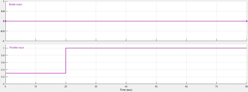
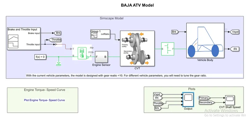 The velocity of the vehicle with respective throttle and brake commands is shown in the figure.
 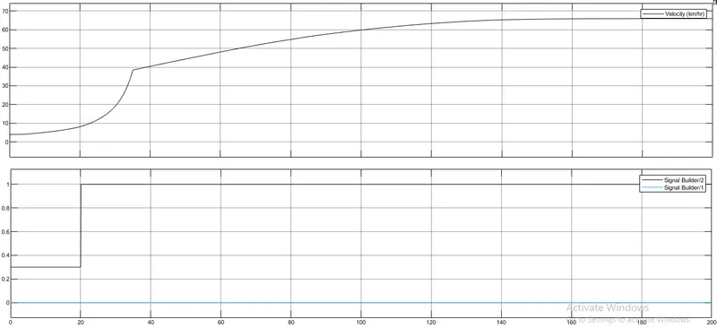 And also the variation of cvt first and second shaft speed is shown in the below figure.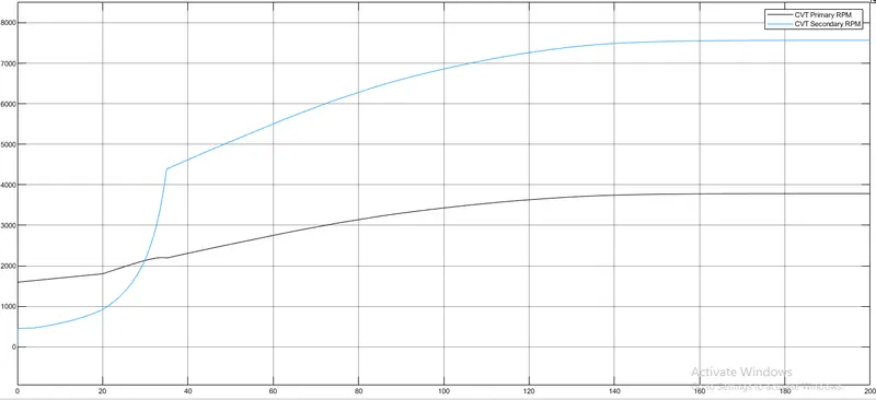
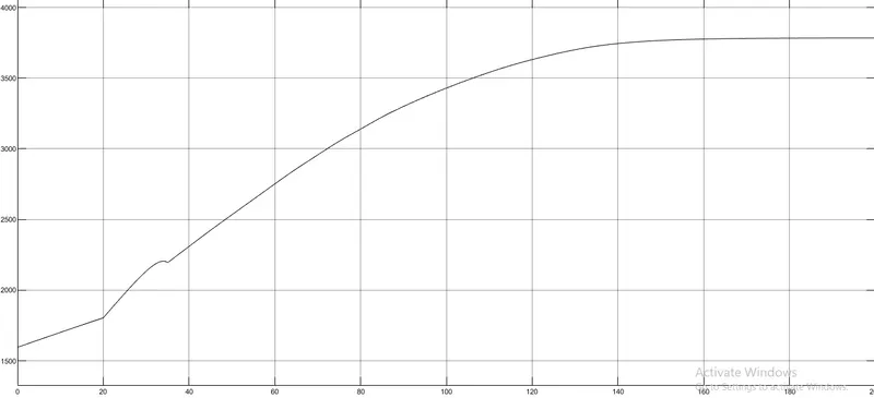
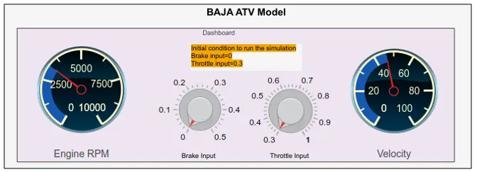
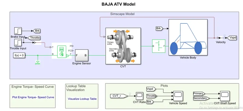
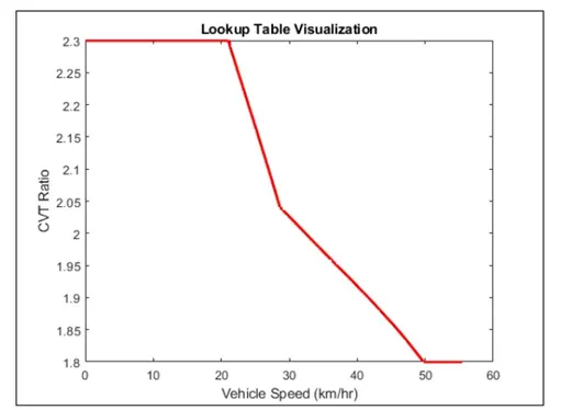
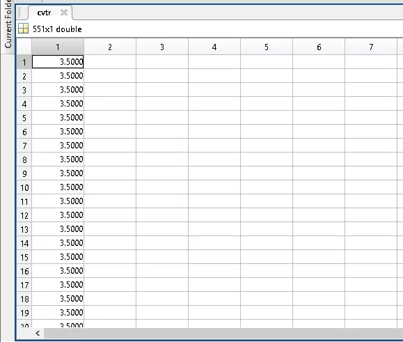
The velocity was fed in to the look up table as input and code was written to get cvt ratio versus velocity
%% Load and simulate the model
cvtModel_data
sim('cvtModel_data')
%% Visualize the lookup table
plot(vehicle_speed,cvtr,'r','LineWidth',2)
xlabel ('Vehicle Speed (km/hr)')
ylabel ('CVT Ratio')
title ('Lookup Table Visualization')
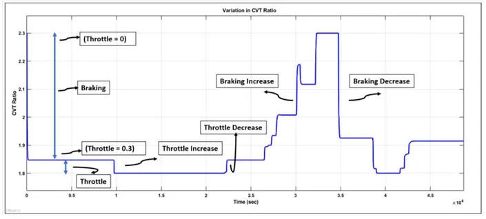
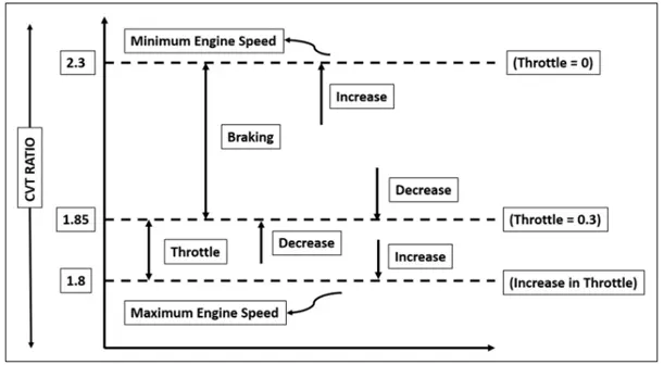
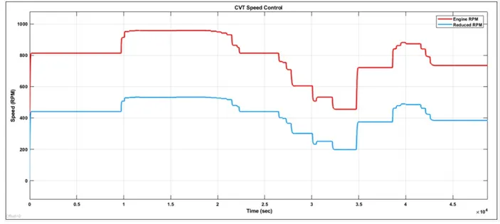
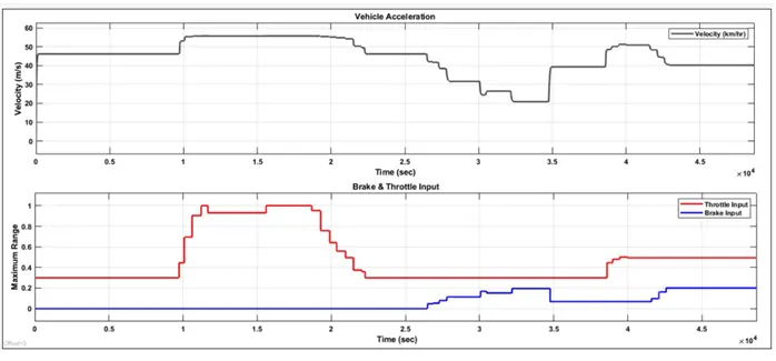
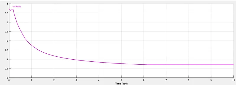 and in closed loop model the ps-lookup table was used in which vehicle speed was fed and gear ratio was determined.The vehicle is made of 4 tyres, 2 front and 2 rear with a vehicle body which contain parameters such as mass,Horizontal distance from CG to front axle,Number of wheels per axle,Horizontal distance from CG to rear axle,CG height above ground ,Gravitational acceleration etc and also inertia ,double shoe brake.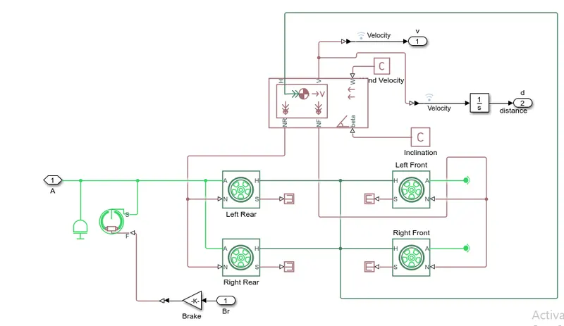
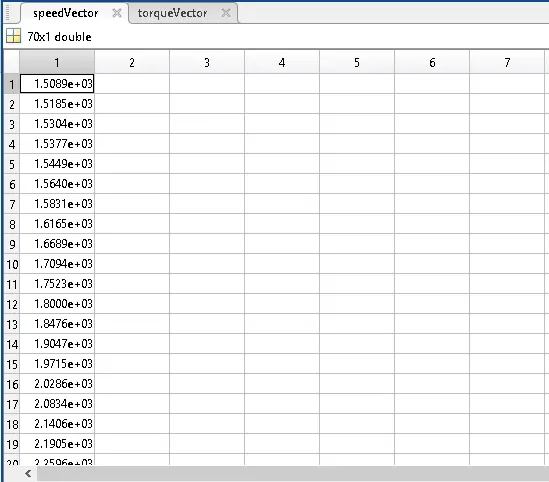
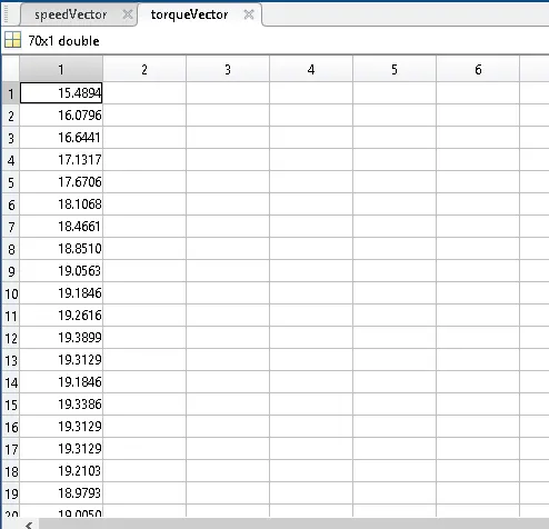
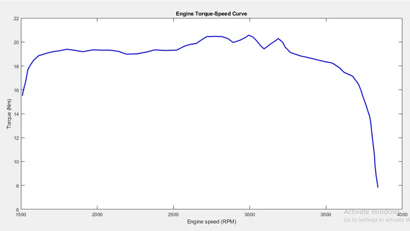
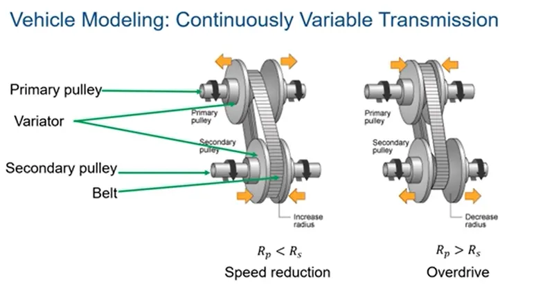
- ATV with cvt data obtained using 1-D lookup table from speed of the engine measured
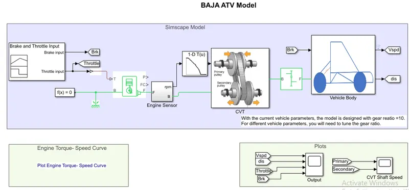
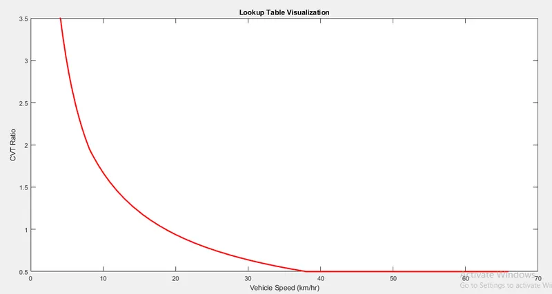 CONCLUSIONS:
The baja atv model was studied and simulated successfully and results were explained.
The speeds are seen tobe proportional to throttle inputs and inversely to braking inputs.
Cvt ratio was inversely proportional throttle inputs and drectly proportional to torque
The closed loop model gives more realistic plots than the open loop model.
REFERENCES:
https://in.mathworks.com/matlabcentral/fileexchange/70576-baja-all-terrain-vehicle-atv-model.
https://github.com/mathworks/BAJA-All-Terrain-Vehicle-Model.
www.atv.info ETC