Project 3- Adding a temperature dictionary to the incompressible icoFoam case to solve the energy equation
Objective:
This work attempts to create a custom icoFoam based solver to solve for a temperature equation and validate the solver through a benchmarking example.
Introduction:
OpenFOAM (Open Field Operation and Manipulation) is a popular open-source CFD toolbox known for its flexibility and extensibility. Unlike commercial software, OpenFOAM allows users to modify the source code and implement custom functionality, making it highly suitable for academic research and specialized industrial applications. Among its many capabilities, OpenFOAM supports the development of custom function objects, which enable users to perform advanced calculations or derive new fields during simulations.
The purpose of this report is to document the implementation and validation of a temperature transport equation in the incompressible laminar cavity flow case in OpenFOAM. This work extends the standard icoFoam solver, which solves the incompressible Navier Stokes equations, by introducing the capability to solve for temperature. The modified solver, named icoTempFoam, accounts for convective and diffusive heat transfer. By adding temperature to the simulation, we can explore thermal effects and heat transport in fluid flows, which is vital for applications in energy systems, heat exchangers, and natural convection problems.
This project involves modifying the solver to incorporate the temperature equation, setting up a case file for the cavity problem with appropriate initial and boundary conditions, and simulating the heat transport alongside the fluid flow. The results are analyzed to confirm that the solver behaves as expected, and a smooth temperature distribution is obtained in the cavity with the specified conditions.
Methodology
Solver Literature
The base icoFoam solver solves the incompressible flow equations for mass and momentum:
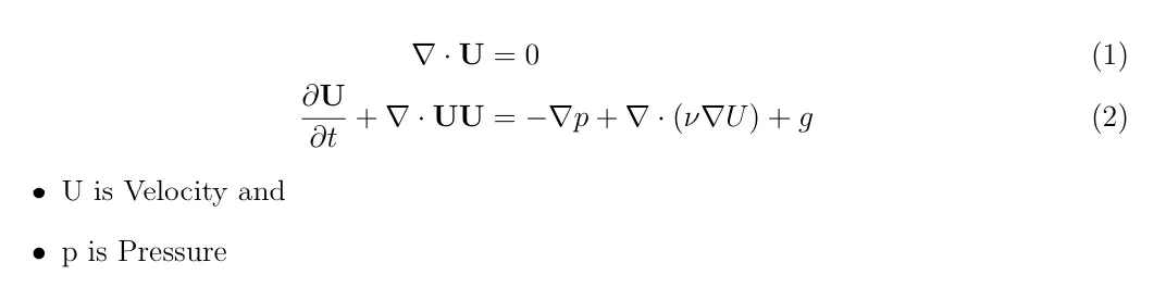
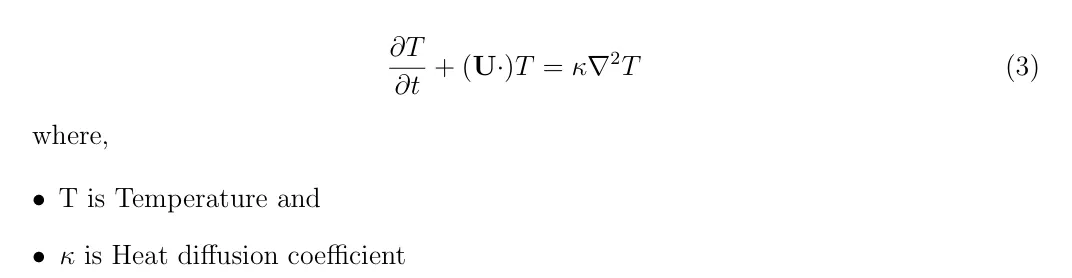
For which, we will be adding the following temperature equation to our solver,
Solver Modification
Now, we will copy the icoFoam solver from the OpenFOAM solver directory to our current user application directory as the new icoTempFoam with the following command:
cp-r $FOAM SOLVER/incompressible/icoFoam icoTempFoam
The solver directory contains the main driver program icoTempFoam.C, createFields.H and Make files. We first rename all the old instances of the solver to the new name
mv icoFoam.C icoTempFoam.C
sed-i ’s/icoFoam/icoTempFoam/g’ *
Similarly, in the Make files, we rename the driver code and specify the directory to save the customized solver to user application directory:
Original Make/files:
icoFoam.C
EXE = $(FOAM APPBIN)/icoTempFoam
Customized Make/files:
icoTempFoam.C
EXE = $(FOAM USER APPBIN)/icoTempFoam
Now, we move onto the main solver modifications. We will first add the additional variables required for the temperature equation in the createFields.H. The additional variable code is given below:
dimensionedScalar kappa
(
"kappa",
transportProperties
);
Info << "Reading field T\n" << endl;
volScalarField T
(
IOobject
(
"T",
runTime.timeName(),
mesh,
IOobject::MUST_READ,
IOobject::AUTO_WRITE
),
mesh
);
Here, we add the dictionary reader for kappa varibale to be read from the transportProperties f ile and the temperature T to be read and solved in the simulation.
We now move on to the main driver code icoTempFOam.C. Here we add the temperature equation (3) through a fvScalarMatrix between the momentum corrector and the PISO loop. The temperature equation code is given below:
// Temperature
fvScalarMatrix TEqn
(
fvm::ddt(T)
+ fvm::div(phi, T)
- fvm::laplacian(kappa, T)
);
TEqn.solve();
Now, we compile the solver using the wmake command and receive the following output:

Figure 1: Solver Compilation
Case Setup
To benchmark this solver, we use the Lid-Driven Cavity case from the icoFoam tutorials directory. The lid-driven cavity flow is a classic benchmark problem in computational fluid dynamics (CFD) that involves simulating fluid motion in a square or rectangular domain driven by the movement of one boundary. For this case, we added the transport of temperature, making it a thermally coupled problem where heat transfer via convection and diffusion is simulated alongside the flow.
First, we navigate to our run directory and copy the cavity case from the tutorials as cavityTemp:
cd $FOAM RUN
cp-r $FOAM TUTORIALS/incompressible/icoFoam/cavity cavityTemp
For the geometry and the mesh, the blockMeshDict file remains the same.
Initial and Boundary Conditions:
The velocity and pressure fields remain the same as the tutorial case. We create a new field T to specify the initial and the boundary conditions for Temperature
0/T:
/*--------------------------------*- C++ -*----------------------------------*\
| ========= | |
| \\ / F ield | OpenFOAM: The Open Source CFD Toolbox |
| \\ / O peration | Version: v2312 |
| \\ / A nd | Website: www.openfoam.com |
| \\/ M anipulation | |
\*---------------------------------------------------------------------------*/
FoamFile
{
version 2.0;
format ascii;
class volScalarField;
object T;
}
// * * * * * * * * * * * * * * * * * * * * * * * * * * * * * * * * * * * * * //
dimensions [0 0 0 1 0 0 0];
internalField uniform 300;
boundaryField
{
movingWall
{
type fixedValue;
value uniform 400;
}
fixedWalls
{
type fixedValue;
value uniform 300;
}
frontAndBack
{
type empty;
}
}
// ************************************************************************* //
As per the given parameters, we set the movingWall to be 400 K, the otherWalls and internalFields to be 350 K.
transportProperties:
The heat diffusion coefficient κ is defined in constant/transportProperties.
/*--------------------------------*- C++ -*----------------------------------*\
| ========= | |
| \\ / F ield | OpenFOAM: The Open Source CFD Toolbox |
| \\ / O peration | Version: v2312 |
| \\ / A nd | Website: www.openfoam.com |
| \\/ M anipulation | |
\*---------------------------------------------------------------------------*/
FoamFile
{
version 2.0;
format ascii;
class dictionary;
object transportProperties;
}
// * * * * * * * * * * * * * * * * * * * * * * * * * * * * * * * * * * * * * //
nu 0.01;
kappa [0 2 -1 0 0 0 0] 0.001;
// ************************************************************************* //
Numerical Schemes:
The fvSchemes file specifies the discretization schemes for the equations. Let’s understand how these work:
Convection Term div(phi,T) (for velocity and temperature):
Scheme used: Gauss upwind
Reasoning:
- The Gauss upwind scheme is first-order accurate and is often chosen for convection terms because it is unconditionally stable for most flow conditions.
- It introduces numerical diffusion, which helps to dampen unphysical oscillations that might arise in high-gradient regions, such as near sharp temperature changes or discontinuities.
- This stability makes it suitable for initial testing or for cases with high Peclet numbers (advection-dominated flows).
Trade-offs
- Numerical diffusion can artificially smooth steep gradients, reducing solution accuracy in cases where precision is critical.
- Lower accuracy compared to second-order schemes because it approximates the temperature gradient based on the upstream value.
Other potential schemes for the convection term include Gauss linear, Gauss limitedLinear, Gauss QUICK
Diffusion Term laplacian(kappa,T) (for velocity and temperature):
Scheme used: Gauss linear corrected
Reasoning:
- The Gauss linear corrected scheme is second-order accurate and provides a good balance between accuracy and stability for diffusion terms.
- Diffusion terms typically involve the second derivative of a field, so higher accuracy is important to avoid smearing physical gradients.
- The corrected option adjusts the diffusion flux based on non-orthogonal cor rections, which is essential for mesh quality that deviates from orthogonality.
- This scheme ensures accurate results for meshes with non-orthogonal or skewed elements, which are common in complex geometries.
Trade-offs:
- Slightly more computationally expensive than simpler schemes like Gauss linear.
Other scheme options include Gauss linear, Gauss harmonic, Gauss limitedLinear
| Scheme | Accuracy | Stability | Best Use Case |
|---|---|---|---|
| Gauss upwind | Low | High | initial testing, convection-dominated flows |
| Gauss linear | High | Moderate (unstable) | Laminar flows with smooth gradients |
| Gauss limited Linear | Moderate | Moderate-High (stable) | Advection-diffusion problems with sharp gradients |
| Gauss linear corrected | High | High | Diffusion terms, especially with non-orthogonal meshes. |
Table 1: Comparison of Schemes
The convection term included in fvSchemes is given below:
divSchemes
{
default none;
div(phi,U) Gauss upwind;
div(phi,T) Gauss upwind; //Convection term
The diffusion term included in fvSchemes is given below:
Solution Parameters:
The fvSolution file is crucial for configuring the solution of the equations and specifying the numerical methods, solver settings, and convergence criteria. The solver parameters and relaxation factors control the behavior of the iterative solvers during the simulation.
As specified, we have used smoothLinear solver for temperature with a tolerance of 1e −07 and a relTol of 0. The following is a breakdown of the reasoning behind the parameters used for the temperature (T) fvSolution file:
Temperature T:
Solver used: smoothSolver
Reasoning:
- The smoothSolver is a general-purpose solver designed for scalar fields like temperature that do not involve complex non-linear terms. It is based on a smoother that solves the system iteratively using a smoother like GaussSeidel.
- This solver is often chosen for diffusion-dominated equations like the tempera ture equation (which includes the Laplacian term) because it converges quickly and is computationally efficient for scalar fields.
- It is particularly useful for problems where the scalar field behaves smoothly and is not highly sensitive to the convective term, which can cause oscillations in higher-order schemes.
- The solver is stable even in cases with low diffusion and can handle smooth, linear systems efficiently.
- Other options include PCG, GAMG
- Since the temperature equation typically has fewer complex terms compared to the momentum and pressure equations, its relaxation factor is generally set to 1.0 (no relaxation). However, if the temperature distribution has sharp gradients or if stability issues occur, relaxation can be reduced.
| Field | Solver | Relaxation Factor | Use Case |
|---|---|---|---|
| Velocity (U) | PBiCG or PCG | 0.7-1.0 | Used for solving momentum equations in incompressible flows. |
| Pressure (p) | PBiCG or GAMG | 0.3-0.7 | Pressure Poisson equation, necessary for incompressible flows |
| Temperature (T) | smoothSolver | 1.0 | Scalar equation, often diffusion-dominated, with high stability. |
Table 2: Summary of Solver Parameters
The fvSolution for temperature is given below:
This completed the case setup. Now, we finally run the simulation with the commands:
• blockMesh: Creates the geometry and the mesh
• checkMesh: Checks if the mesh has been properly implemented
• icoTempFoam: Runs the Solver
• touch cavTemp.foam: Creates a file to load in Paraview
We can confirm that the temperature is begin solved by looking at the icoTempFoam log below:
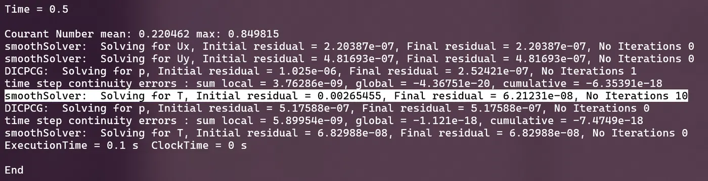
Figure 2: Lid Driven Case Simulation
Results and Observations
Once the simulation is done, we post-process the results in Paraview. The Temperature T variable loads seamlessly, the initial and the final contours are shown below:
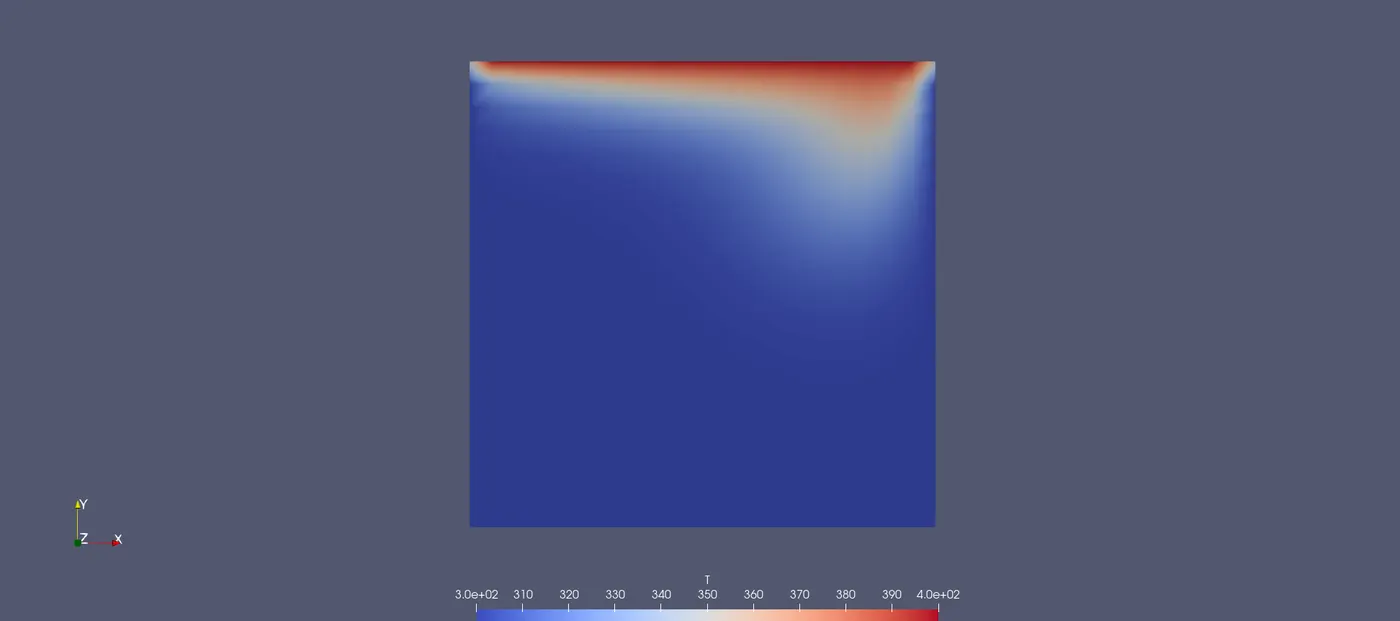
Figure 3(a) First Time Step
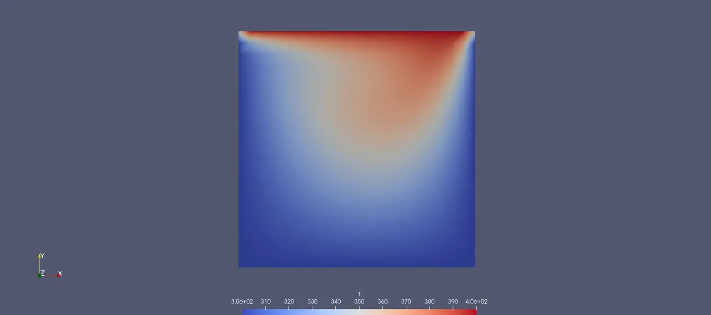
Figure 3(b) Final Time Step
Temperature Distribution:
• The initial temperature distribution, as shown in Fig. 3(a), exhibits a uniform temperature profile across the computational domain. At the start of the simu lation, the temperature is initialized to a constant value, representing the initial condition before any fluid flow or thermal diffusion occurs. This initial uniformity in temperature serves as the baseline for observing how the temperature field evolves over time due to the influence of the fluid velocity and thermal diffusivity.
• From the final temperature contours, it is evident that the fluid flow, represented 12 by the velocity field, has influenced the distribution of temperature. The regions where the fluid moves faster exhibit lower temperature values due to the convective heat transfer. Conversely, the regions where the fluid velocity is slower or stagnant have higher temperatures, indicating the accumulation of heat in those areas due to slower diffusion.
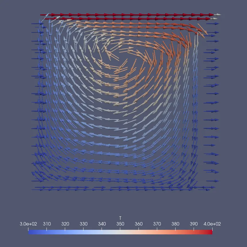
Figure 4: Glyph Representation using Arrow Attributes
Key Observations:
• Thermal Boundary Layers: At the walls or boundaries of the domain, thermal boundary layers form due to the no-slip condition imposed on the fluid velocity. These layers are thicker in regions with lower fluid velocity, where thermal diffusion plays a more significant role.
• Effect of Flow: The velocity field strongly influences the temperature distribution. Higher velocity regions experience more rapid thermal transport, causing a more uniform temperature distribution, whereas lower velocity regions retain heat for longer periods, creating localized temperature pockets.
• Steady-State Behavior: After a sufficient number of iterations, the temperature f ield reaches a quasi-steady state where the heat flux due to convection and diffusion becomes balanced. This is indicated by the stabilization of temperature contours, with no further significant changes in the temperature distribution over time.
Conclusion
This project involved the development and implementation of a custom solver icoTempFoam in OpenFOAM to simulate the coupled flow and heat transfer in a lid-driven cavity. The development of the custom solver was successful, and the validation through the bench marking case confirmed its accuracy. By modifying OpenFOAM’s existing solvers and implementing the necessary changes to incorporate temperature transport, this project expanded the capability of OpenFOAM for simulating heat transfer in confined fluid do mains.
The solver is now capable of handling coupled velocity and temperature fields in transient conditions, which opens up opportunities for simulating more complex thermal f luid dynamics problems. This work also highlights the importance of validating custom solvers against benchmark cases to ensure the correctness of numerical results. The methodology can be applied to a wide range of fluid dynamics and heat transfer problems in engineering, particularly in thermal management and energy systems. Future work could include extending the solver to include turbulence models, multiphase flows, or more complex thermal boundary conditions.
Note: The final report with the entire code has been typeset and written in LaTeX and has been attached to this submissison.