Project 3

Alternatives to PCBs include wire wrap and point to point construction, both once popular but now rarely used. PCBs
manufacturing and assembly can be automated. Electronic
the work of layout. Mass-producing circuits with PCBs is
layout only has to be done once. PCBs can also be made
PCBs can be single-sided one copper layer, double-sided two
component density because circuit traces on the inner layers would otherwise take up surface space between components. The rise in popularity of multilayer PCBs with more than two, and especially with more than four, copper planes was concurrent with the adoption of surface mount technology. However, multilayer PCBs make repair, analysis, and field modification of circuits much more difficult and usually
2. Problem Description: A PCB board, library files, and traces are imported to create the model. The model is first solved for conduction only, without the components and then solved using the actual

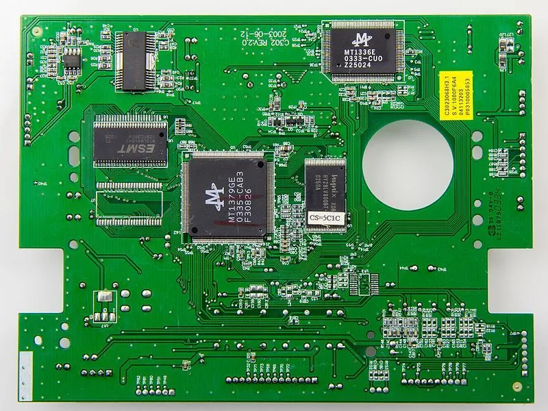
• Modeling: Files are provided with this
1. Create a new project 2. Import board layout *bdf& *.ldf (The board and the
associated library files have to be chosen at this step and
the trace file can be imported later.) 3. Form the nonconformal assembly 4. Import ECAD file (*.anf) A1.anf can be found in the folder
containing the input files downloaded for his tutorial. 5. Once the import process is completed, you can edit the
layer information in the Board layer and via information panel (metal layers are pure Cu and the dielectric layers
6. Enter the layer thickness as shown in the table below.
Layer No. Layer Thickness (mm)
7. Specify Grid density by size (0.508 mm X 0.508 mm) Conduction only model: Thermal conduction is the transfer of internal energy by microscopic collisions of particles and the movement of electrons within a body. The colliding particles, which include molecules, atoms, and electrons, transfer disorganized microscopic kinetic and potential energy, jointly known as internal energy. Conduction takes place in all phases solid,
bodies and the properties of the conductive interface through
Heat spontaneously flows from a hotter to a colder body. For example, heat is conducted from the hotplate of an electric
temperature becoming more uniform In conduction, the heat flow is within and through the body
combination of conduction and thermal radiation. In convection, the internal energy is carried between bodies by a
propagation and collisions of phonons, and diffusion and collisions of free electrons. In gases and liquids, conduction is due to the collisions and diffusion of molecules during their random motion. Photons in this context do not collide with
radiation is conceptually distinct from heat conduction by microscopic diffusion and collisions of material particles and phonons. But the distinction is often not easily observed unless the material is semi-transparent 3. Meshing & BC setting 1.consider aboard without any components. Make all objects
BOARD_OUTLINE.1 object.
VIEW MORE
components in the domain to see the analysis on the board
2. Select the cabinet and select Autoscale from the Edit
Cabinet (cabinet. 1] Info Geometry Properties
Notes
Prism
Local coord system
Specify by: Start/ end xs-12.57300 mm xE 162.039 mm ys -105.5149 mm y 4.3559 mm z5 -0.025399 mm ze 15.02664 mm
Geom
Prism
Start /end
3
V Apply
Reset
Edit
z5|-0.0253 mm
zE|15.028 mm

We have used an auto-scale option for making the size of the board and cabinet at the same. 3.Min z: Temperature from the External conditions dropdown list, and keep the ambient temperature (20°C).
Moving
Effective thickness
Walls (cabinet_default_side_minz] Info Geometry Properties Notes Wall type: Stationary Symmetry
Material Wal thickness Ommy Solid material Beaut External material default Internal material defaul Thermal specification External conditions Temperature
VIEW MORE
Edit
Transient Inner surface radiation
Fix values
✓ Update
New
Reset Cancel
Delete Help
Copy from
Done
X

shown above and the considered ambient temperature on the min z wall side is 20°C. 4.Max z: specify a Heat flux of 20000 W/m2 in the Thermal
Walls (cabinet_default_side_maxz] Into Geometry Properties Notes Wall type: Stationary Symmetry
Moving
Effective thickness
Wall thickness 0 mm Solid material default External material default Internal material faut Thermal specification External conditions Heat flux
Heat flux
Profile
20000 W/m2 Edit
Fix values
shown above and the considered heat flux is 20000 W/m^2. 5. The rest of the sides are insulated. The board will be simulated using a conduction-only model. E- Model
Cabinet (cabinet. 1] - Materials
Into Geometry Properties Notes Cabinet
Waltype Properties - small components
Minx Default
Edt HU BOARD_OUTUNE. 1
Detour cabinet_delault_side_mirz cabinet_default_side_maxz
Max y Default
Update
Reset
Done
x Cancel
Heb

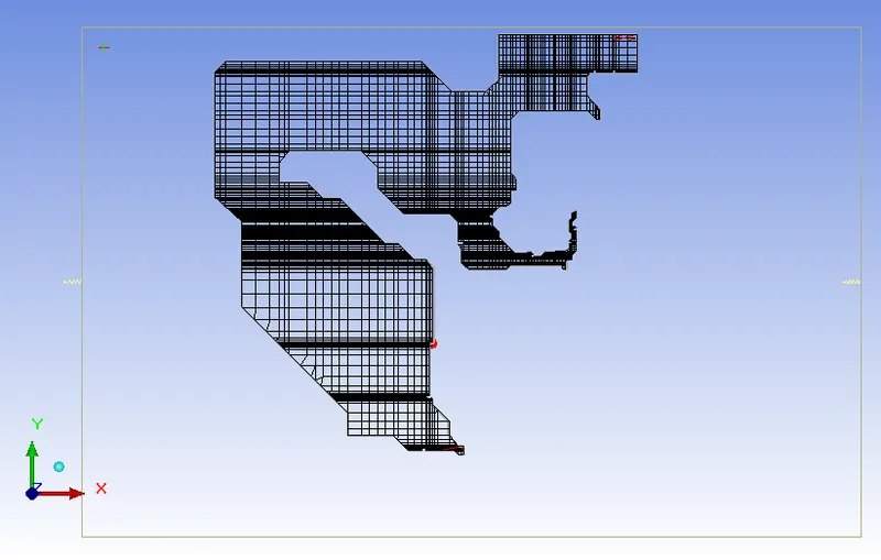
The remaining walls were considered as the insulated in the x and y directions and the z-direction, we have used the conduction model. 6. Generate mesh. Specify a Max element size for X, Y, and Z as 2.032, 2.032, and 0.05 mm respectively, and a Minimum
VIEW MORE
Mesh generation is the practice of creating a mesh, a subdivision of a continuous geometric space into discrete geometric and topological cells. Often these cells form a simplicial complex. Usually, the cells partition the geometric input domain. Mesh cells are used as discrete local approximations of the larger domain. Meshes are created by computer algorithms, often with human guidance through a GUI, depending on the complexity of the domain and the
accurately captures the input domain geometry, with highquality (well-shaped) cells, and without so many cells to
also be fine (have small elements) in areas that are important for the subsequent calculations
Mesh control Num elements: 137268 Num nodes: 146080 Settings Display Quality
E Load. Generate... Mesh type Mesher-HD Mesh units mm Concurrency
Max element size Minimum gap FX 2.032 Y 2.032
zr0.01 mm
VIEW MORE
Global
Local Multi-level
Options Misc Normal
Mesh parameters Min elements in gap Min elements on edge Max size ratio
Allow stair-stepped meshing Mesh assemblies separately Set uniform mesh params
Use average Keep XYZ max sizes
Mesh generation Meshes are used for rendering to a computer screen and for physical simulation such as finite element analysis or computational fluid dynamics. Meshes are composed of simple cells like triangles because, e.g., we know how to perform operations such as finite element calculations (engineering) or ray tracing (computer graphics) on triangles,
on complicated spaces and shapes such as a roadway bridge. We can simulate the strength of the bridge, or draw it on a computer screen, by performing calculations on each triangle and calculating the interactions between triangles.
VIEW MORE

4. Numerical setting: Basic parameters: Flow & Radiation is off
Advanced
Basic parameters General setup Defaults Transient setup Variables solved
Flow (velocity/pressure) Temperature
On Off
Surface to surface radiation model Discrete ordinates radiation model Ray tracing radiation model
Options E Options
Options
Flow regime
Turbulent zero equation
Natural convection
Y
9.80665 m/s
Accept
Reset
X Cancel
Help
In the Basic parameters, we have considered the flow, and radiation was turned off and the flow region was considered to be laminar.
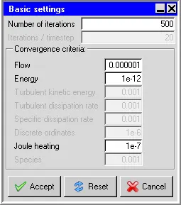
Set no of iterations 500 and convergence criteria for energy
Number of iterations
Convergence criteria Flow
|
Turbulent kinetic energy Turbulent dissipation rate Specific dissipation rate Discrete ordinates
0.001 0.001 0.001
es
V Accept
Reset

and coming to the convergence criteria the flow was set to 0.000001 and energy was 1e-12, and the turbulent kinetic
Dave Bds
From the residual plot, it is clear that the simulation has reached the converged stage and also obtained the converge, and they are no fluctuations in the plot. Temperature Linear solver: F cycle is selected for Type Enter
reduction tolerance In applied mathematics, discretization is the process of transferring continuous functions, models, variables, and
numerical evaluation and implementation on digital computers. The discretization scheme properties were set accordingly as
Discretization scheme
Standard
Body Force
PRESTO
Second Second Second
Secondary gradient
Momentum Temperature Turbulent kinetic energy Turbulent dissipation rate Specific dissipation rate Discrete ordinates
First First First First
Second Second Second
Under-relaxation
Pressure
Temperature Viscosity Body forces Turbulent kinetic energy Turbulent dissipation rate Specific dissipation rate Joule heating potential
1.0 0.8 0.8 0.8 1.0
Linear solver
Termination Residual reduction
criterion tolerance
Stablization
None
1e-6 None

Momentum Temperature Turbulent kinetic energy Turbulent dissipation rate Specific dissipationale Joule heating potential
ex
F
07 None
-
Linear solver advanced controls
2
-1
Precision
Double
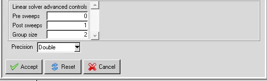
Enter a value of 1e-6 for both the Termination criterion and
Select Double for the solver Precision.
Linear solver advanced controls Pre sweeps
0 Post sweeps 1 Group size
2 Precision Double
-
Accept
Reset
x Cancel
means that they will be represented in a 64-bit system. So
Save the model: ANSYS Icepak will save the model for you automatically
model (including the mesh) as well. If we exit ANSYS Icepak before you start the calculation, we will be able to open the
VILVMORC
Icepak will simply overwrite your job file when it saves the
General setup
Advanced
Results
ID PCLO1 Type New Restart Jocb0025
B Select Interpolated data
Full data Solver options
Disable radiation Disable varying joule heating Disable flow and turbulence equations for restarts Sequential solution of flow and energy equations Temperature secondary gradients for skewed meshes Alternative secondary gradient formulation at walls Coupled pressure-velocity formulation Options
Start solution
Dismiss
☆ Cancel
There are no universal metrics for judging convergence, a good indicator is when the solution no longer changes with more iterations, and when the residuals have decreased to a certain degree. The default criterion is that each residual will
residual, for which the default criterion is 10^-7. It is a good
levels but also by monitoring relevant integrated quantities.
General setup
Advanced
Results
Write overview of results when finished Write report when finished
Write XML-based report when finished Workflow data
CFD Post/Mechanical data
Auto-save interval
Compress solution after reporting Write interpolated restart data file Write full restart data file Wnte electric current density vector Create heat flux vectors in CFD Post Export Nastran =
Start solution
Dismiss
Cancel
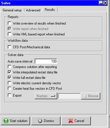
ANSYS Icepak will begin to calculate a solution for the model, and a separate window will open where the solver will print the numerical values of the residuals. ANSYS Icepak will also open the Solution residuals graphics display and control window, where it will display the convergence history for the calculation. 5. Examine and post-process the results: View the traces in three different ways, i.e. single color, color by layer, or color by trace
copper is its color it will be green. One famous example of copper oxidation is the Statue of Liberty. PCB copper platingalso known as copper coating, copper finish, and the surface finish has two essential functions: 1. To protect the exposed copper circuitry 2. To provide a solderable surface when assembling soldering components to the PCB. A variety of PCB copper plating options exist, and each carries its advantages and
TA
A single color for the trace image was shown above. the color by layer
Han
Color by layer for the trace image was shown above. color by trace
EL

Color by trace for the trace layout image was shown above.
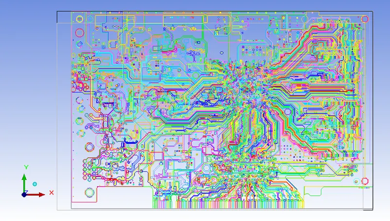
developments, but the one thing that remains unchanged is the basic construction of a PCB. A printed circuit board can have a single layer, or it may vary from 1 to 20 layers depending upon the application for which it is designed. Twisted Traces is a leading manufacturer of PCBs, which provides PCBs in 1-20 layers (FR-4, FR- 406, 370 HR), and in 1- 2 Layers (Rogers, Aluminum/Copper Base, Teflon). There
1. Inner Layers
Also referred to as internal layers in multilayer PCBs, the
pour technique, which helps a lot in the layer-to-layer bonding process. The copper pour helps reduce the
copper weight and thickness are customizable and depend on the application requirements. The weight of copper in the layer determines the minimum trace width
2. Outer Layers
technique or soldering into the through-holes. The outer layer consists of a copper foil, which is electroplated with copper. This is done to increase the thickness and add copper to the through-hole barrels. The thickness of the finished copper is customizable depending upon the
Metal traces base layer-1
are
00.00
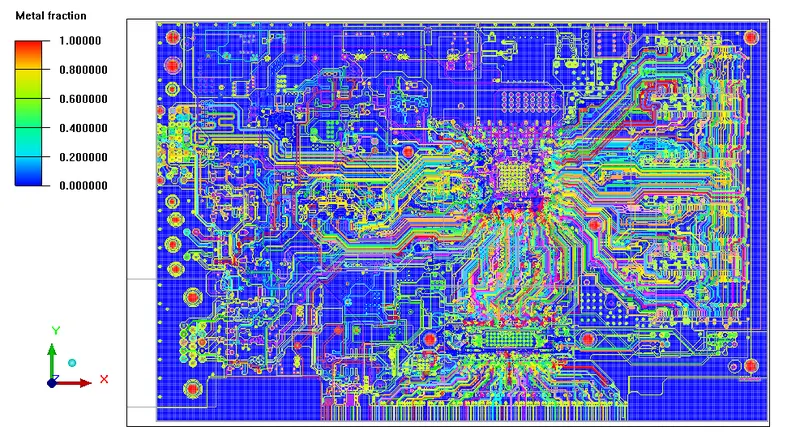
representation of the legend shown the amount of the metal
Metal traces base layer-2
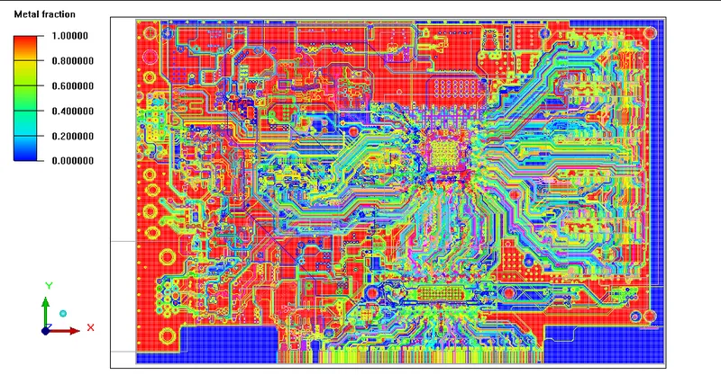
The metal traces for the layer-2 was shown above and the representation of the legend shown the amount of the metal trace on the board.

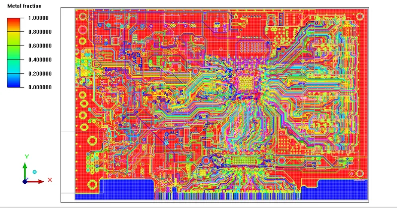
The metal traces for the layer-3 was shown above and the representation of the legend shown the amount of the metal trace on the board. Metal traces base layer-4
We
The metal traces for the layer-4 was shown above and the representation of the legend shown the amount of the metal trace on the board. Metal traces base layer-5
The metal traces for the layer-5 was shown above and the representation of the legend shown the amount of the metal trace on the board. Metal traces base layer-6
The metal traces for the layer-6 was shown above and the representation of the legend shown the amount of the metal
Metal traces base layer-7
EVENS
The metal traces for the layer-7 was shown above and the representation of the legend shown the amount of the metal
VIEW MORE
The plane cut Point and normal. Make sure that PX, PY, PZ are 0, 0, and 0.78232, respectively, and NX, NY, and NZ are 0, 0, and 1, respectively.
Active -Plane location Set position Point and normal
Update POPYOPZ 0782:
A0B NX ONYO NZ 1 1000075
Enable clipping
Stal 00 End Step 16 Delay (ms
Witetotle Loop node
10 24
p Show contours
Show vectors Show particle haces
P
Parameters
eters Parameters
The cut plane was generated concerning the required plane and the cut plane was considered according to the point of normal and the respective dimension was considered in the
Temperature contour
Temperature (9
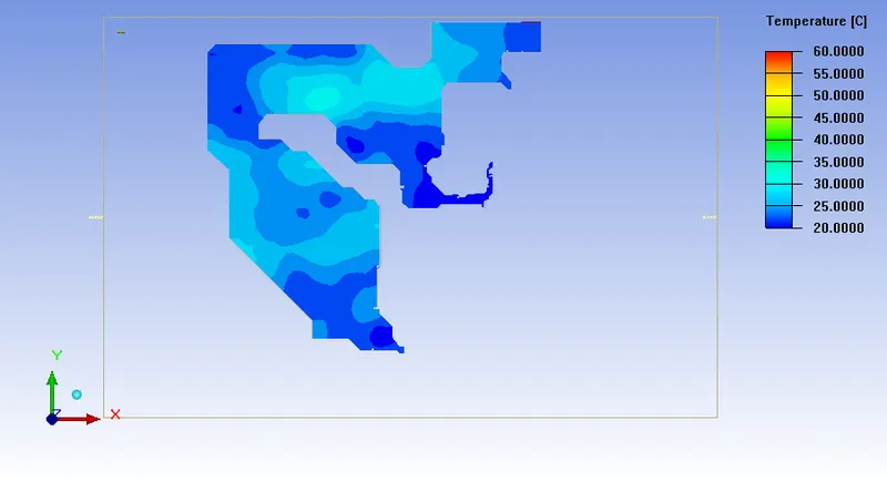
opposite is true for the low-temperature regions, i.e. maximum trace concentration leads to low temperatures. This is expected as the copper content is directly proportional to the trace concentration. It is worth noting that if a compact or detailed PCB were used instead of the traced PCB, one would obtain a fixed temperature for the entire mid-plane and this fixed temperature would be different from the average temperature of the traced PCB on the same plane. The initial temperature was at a temperature of 20°C and the final temperature has reached a maximum temperature of
The animation for the temperature profile on the PCB board.
animation for the temperature profile o...
Watch later Tomat

animation for the temperature profile on the PCB
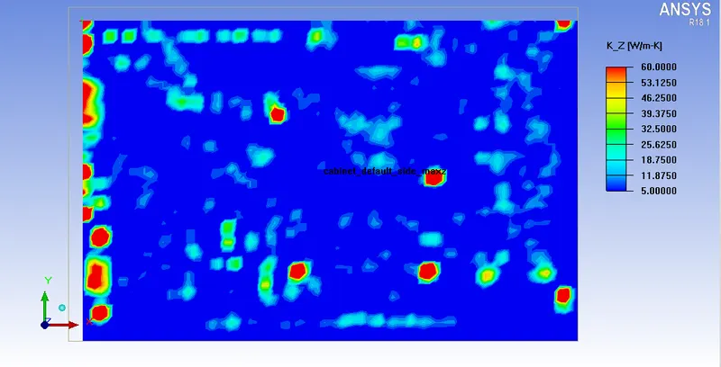
The spatially varying non-uniform conductivity of the board can also be viewed during post-processing. The conductivities in the three directions K_X, K_Y, and K_Z are available as post-processing variables with plane cuts and object faces.
and has reached a final temperature of 60W-m/k.
Forced convection is a mechanism or type of transport in
pump, fan, suction device, etc. Alongside natural convection,
methods of heat transfer and allows significant amounts of heat energy to be transported very efficiently. 3. Meshing & BC setting: Put the actual components back into the model.
OREFDE-HEATSINK BROZ|1965X300
The components were kept back into geometry which is
temperature that has been obtained in the domain. Highlight the two wall objects created for the "conduction only" model and drag them into the Inactive folder. Click on the Cabinet and Autoscale it from the Edit window.
Notes
Cabinet (cabinet. 1] Info Geometry Properties Shape
Prism Local coord system
Specify by: Start /end *S -12.57300 mm x 162.039 mm ys -1055149 mm E 4.3559 mm 25 0.025399 mm ZE 15.02664 mm
Fix values
VIEW MORE
Apply
Reset
Edit
yS-105.51 mm y 4.3559 mm 25|-0.0253 mm 215,028 mm
board and cabinet at the same.
E
Malenel:
BOARD_OUTLINE 1 cabinet_default_side_mina
Info Geometry Properties Notes
Waltype Properties Min pering
t Maxx Opering a t Ming Wall Edt Mary Wall Edt Mina Wall Edt Masz wol
Edt r Fie values
cabine_default_side_miny cabinet_default_side_max
Update
Reset
Done
x Cancel
Help
Assign an X Velocity of -1.5 m/s for Max x side of the cabinet.
Openings (cabinet_default_side_maxx] Info Geometry Properties Notes Thermal specification Temperature
ambient CE
Transient
External radiation temp ambient Flow specification
Static pressure ambient N/m2
Transient
Edit
Y Velocity
Om
Transient
Species
Edit
Fix values
We have assigned a value of -1.5m/sec in the x-direction of the opening which has been provided in the cabinet facing. Generate mesh. Specify a Max element size for X, Y, Z as 9,5, 7, and 0.7 mm respectively. Mesh generation is the practice of creating a mesh, a
geometric and topological cells. Often these cells form a simplicial complex. Usually, the cells partition the geometric input domain. Mesh cells are used as discrete local approximations of the larger domain. Meshes are created by computer algorithms, often with human guidance through a GUI, depending on the complexity of the domain and the type of mesh desired. The goal is to create a mesh that accurately captures the input domain geometry, with high
make subsequent calculations intractable. The mesh should also be fine (have small elements) in areas that are important for the subsequent calculations
Num elements: 222184 Num nodes: 234761 Settings Display Quality
Load... | Generale... Mesh type Mesher-HD Mesh units mm Concurrency Max element size
Minimum gap x 10.0007874 m
Misc
Global Local Multi-level Options Mesh parameters Normal Min elements in gap Min elements on edge Max size ratio
Allow stair-stepped meshing Mesh assemblies separately Set uniform mesh params
VIEW MORE
Meshes are used for rendering to a computer screen and for physical simulation such as finite element analysis or computational fluid dynamics. Meshes are composed of simple cells like triangles because, e.g., we know how to perform operations such as finite element calculations (engineering) or ray tracing (computer graphics) on triangles, but we do not know how to perform these operations directly on complicated spaces and shapes such as a roadway bridge. Mesh generation:
VIEW TURL
computer screen, by performing calculations on each triangle and calculating the interactions between triangles.
Basic parameters toggle on the Flow button. Keep and choose Turbulent and Zero equation for the flow regime
Basic parameters General setup Defauts
Transient setup
Advanced
Temperature
On Off
Suface to surface radiation model C Discrete ordinates radiation model
Ray tracing radiation model
Options Options Options
Natural convection
0 m/s2
In the Basic parameters, we have considered the flow, and radiation was turned on and the flow region was considered to be Turbulent. set no of iterations 500 and convergence criteria for energy
v
Basic settings Number of iterations Iterations / timestep - Convergence criteria
1
Turbulent kinetic energy Turbulent dissipation rate Specific dissipation rate
0.001 0.001 0.001
Joule heating
Accept
Reset

The total number of iteration was set to be 500 iterations
0.00001 and energy was 1e-12, and the turbulent kinetic energy and turbulent dissipation rate were 0.001
Orrom CCM From the residual plot, it is clear that the simulation has
Temperature Linear solver: F cycle is selected for Type Enter 1e-6 for both the Termination criterion and Residual reduction tolerance In applied mathematics, discretization is the process of transferring continuous functions, models, variables, and equations into discrete counterparts. This process is usually carried out as a first step toward making them suitable for numerical evaluation and implementation on digital
The discretization scheme properties were set accordingly as shown below
Advanced solver setup
Pressure
Standard
Second
Body Force
PRESTO
Secondary gradient
Temperature Turbulent kinetic energy Turbulent dissipation rate Specie dissipationale Discrete ordinates
First First First First
Second Second Second Second Second
Turbulent kinetic energy
0.8
Specific dissipation rate Joule heating potential
0.8
10 Termination
Linear solver
Residual reduction
tolerance
Stablization
criterion
1c6
100 None
7
Turbulent kinetic energy Turbulent dissipation rate
Joule heating potential
0.7 None
Linear solver advanced controls
2
Enter a value of le-6 for both the Termination criterion and Residual reduction tolerance and the F cycle is was selected. Select Double for the solver Precision.
Linear solver advanced controls Pe sweeps Post sweeps 1
Precision Double
Accept
Reset
Single precision means that the floating-point numbers will be represented in a 32-bit system whereas double-precision means that they will be represented in a 64-bit system. So
Save the model. ANSYS Icepak will save the model for you automatically before it starts the calculation, but it is a good idea to save the model (including the mesh) as well. If we exit ANSYS Icepak before you start the calculation, we will be able to open the job that we saved and continue with our analysis. If we start the calculation in the current ANSYS Icepak session, ANSYS
Enable Sequential solution of flow and energy equations
General setup
Advanced
Results
Type
New Restart pcb0025
Interpolated data
Disable radiation Disable varying joule heating Disable flow and turbulence equations for restarts Sequential solution of flow and energy equations Temperature secondary gradients for skewed meshes Alternative secondary gradient formulation at walls Coupled pressure-velocity formulation Options
Dismiss
Cancel
Solve the model.
General setup
Advanced
Results
ID Type
pcb01
New Restart Jpcb0025
Interpolated data
r
Disable radiation Disable varying joule heating Disable flow and turbulence equations for restarts Sequential solution of flow and energy equations Temperature secondary gradients for skewed meshes Alternative secondary gradient formulation at walls Coupled pressure-velocity formulation Options
VIEW MORE
Start solution
Dismiss
There are no universal metrics for judging convergence, a good indicator is when the solution no longer changes with more iterations, and when the residuals have decreased to a
be reduced to a value of less than 10^-3 except the energy residual, for which the default criterion is 10^-7. It is a good idea to judge convergence not only by examining residuals
General setup
Advanced Results
Write overview of results when finished
Write XML-based report when finished
CFD Post/Mechanical data
Compress solution after reporting
Write full restart data file Write electric current density vector Create heat flux vectors in CFD Post
ANSYS Icepak will begin to calculate a solution for the model, and a separate window will open where the solver will print the numerical values of the residuals. ANSYS Icepak will also open the Solution residuals graphics display and control
5. Examine and post-process the results: View the traces in three different ways, i.e. single color, color by layer, or color by trace All traces found on external PCB layers as opposed to internal layers must be protected from the elements. If left
finish has two essential functions: 1. To protect the exposed copper circuitry
carries its advantages and
options exist, and each disadvantages.
200
A single color for the trace image was shown above.
Color by layer for the trace image was shown above.
Color by trace for the trace layout image was shown above. View the fraction of metal traces based on the grid density There have been a lot of improvements and advancements in
to deciding its board density, PCBs have seen a lot of
VIEW MORE
have a single layer, or it may vary from 1 to 20 layers depending upon the application for which it is designed. Twisted Traces is a leading manufacturer of PCBs, which provides PCBs in 1-20 layers (FR-4, FR- 406, 370 HR), and in 1- 2 Layers (Rogers, Aluminum/Copper Base, Teflon). There are two main layers on any PCB. They are as follows:
Also referred to as internal layers in multilayer PCBs, the inner layers can be fabricated with a positive or negative
pour technique, which helps a lot in the layer-to-layer bonding process. The copper pour helps reduce the etchant during the PCB manufacturing process. The copper weight and thickness are customizable and depend on the application requirements. The weight of
and spacing that can be manufactured.
electronic components either by surface mounting
layer consists of a copper foil, which is electroplated with copper. This is done to increase the thickness and add copper to the through-hole barrels. The thickness of the finished copper is customizable depending upon the
2010
TELE
600.00
The metal traces for the layer-1 was shown above and the representation of the legend shown the amount of the metal trace on the board. Metal traces base layer-2
The metal traces for the layer-2 was shown above and the representation of the legend shown the amount of the metal trace on the board.
PS
BOS
The metal traces for the layer-3 was shown above and the representation of the legend shown the amount of the metal trace on the board. Metal traces base layer-4
VIEW MORE
The metal traces for the layer-4 was shown above and the representation of the legend shown the amount of the metal trace on the board. Metal traces base layer-5
The metal traces for the layer-5 was shown above and the
Metal traces base layer-6
The metal traces for the layer-6 was shown above and the representation of the legend shown the amount of the metal trace on the board. Metal traces base layer-7
The metal traces for the layer-7 was shown above and the representation of the legend shown the amount of the metal
The plane cut Point and normal. Make sure that PX, PY, PZ are 0, 0, and 0.78232, respectively, and NX, NY, and NZ are O, O, and 1, respectively.

Nome cul2
NXO NYLONZ 11
Minz 254-OCE
Max
2
015026
Start 00 End Step 16 Delay (m)
Witetotle Loop node
10 24
Show contouts Show vector Show particle traces
Parameters Parameters parameters
The cut plane was generated concerning the required plane and the cut plane was considered according to the point of normal and the respective dimension was considered in the
Temperature contour
The temperature distribution at the top of the surface of the board was shown above. Two hot spots are identified underneath the high heat flux components, and the initial temperature was at 13.3°C and the maximum temperature has reached a temperature of 106.7°C Animation for the temperature contour on the PCB
The temperature distribution profile on the PCB
K_Z contour:

The spatially varying non-uniform conductivity of the board can also be viewed during post-processing. The conductivities
post-processing variables with plane cuts and object faces.
case, since we chose not to model the layers separately there
we can see the thermal conductivity was initial at 25W-m/k and has reached a final temperature of 200W-m/k. 6. Joule/Trace Heating Since PCB traces have electrical resistance, they heat up as current flows through them. Modeling this phenomenon will provide us with an accurate prediction of the temperature distribution in the PCB, which can be important.