Project 2 Thermal modeling of battery pack

AIM:
To create a MATLAB model for a for a 10 cell series lithium ion battery model and simulate the thermal effects and compare life cycle performance at various temperatures, charge & discharge rates.

SIMULINK MODEL:

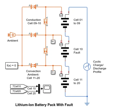
• This example shows how to simulate a battery pack consisting of multiple series connected cells efficiently.
• It also shows how a fault can be intorduced into one of the cells to see the impact on battery performance and cell temperatures. for efficiency, indentical series-connected cells are not just simply modeled by connecting cell models in seriers.
• Instead,a single cell is used, and the terminal voltage is scaled up by the number of cells.
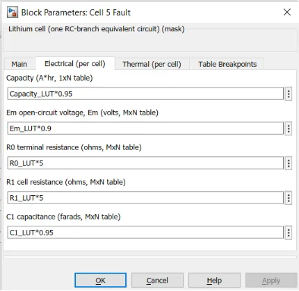
• The fault is represented by changing the parameters for the cell 10 facult subsystem, reducing both capacity and open-circuit, voltage and increasing the resistance values.

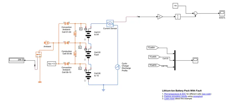
• Lithium ion battery pack with fault is to simulate a battery pack consists of multiple cells connected in series efficiently it also shows how a fault can be introduced into one fo the cells to the impact on battery performance and cell temperatures, for efficiency the identical series connected cells are not just simple model by connecting cell models in seres.
• instead single cell is used, and the terminal coltage is scaled up by the number of cells.
• The fault is represented by changing the parameters for the cell 5 subsystem, reducing both the capacity and open circuit voltage and increasing the resistance values.
  

CELL 01 TO 04 SUBSYSTEM:

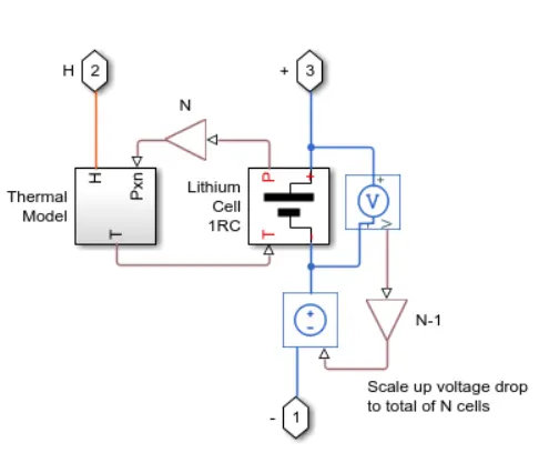
• The cell subsystem basically consists of a thermal model and lithium cell 1RC block which calculate the temperature and thermal effect for cells and overall calculate for the battery pack.
• the block which are inside the cell subsystems are PS gain block which multiplies the input physical signals by a constant i.e. y=c*gain.another block are voltage sensor and current-voltage source.
• the voltage sensor block represents an ideal voltage sensor, this is a dvice that converts voltage mesure between any electric connection into a physical signal proportional to the voltage.
• the current-voltage source represents an ideal voltage source that is powerful enough to maintain the specified voltage at its output regardless of the current passing thorugh it.
• the output voltage is V=Vs, where Vs is the numeric value represents at the physical signal port.

Thermal Behavior and Fault Setup:
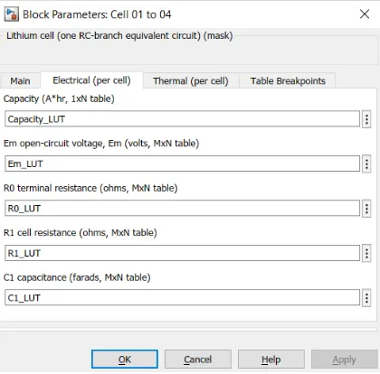
for cell 1 to 4 :

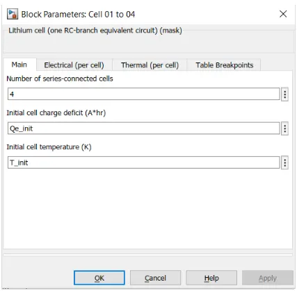
no of cells connected in series = 4
initial temperature = 299.1 k

For cell 5:

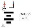
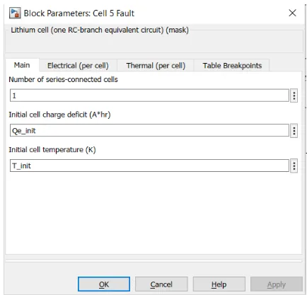
number of cells connected in series = 4.
initial temperature = 299.1 k

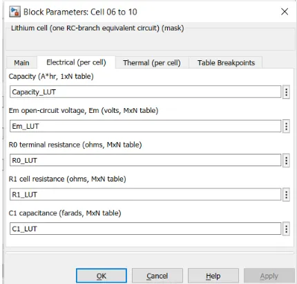
For cell 6 to 10:

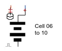
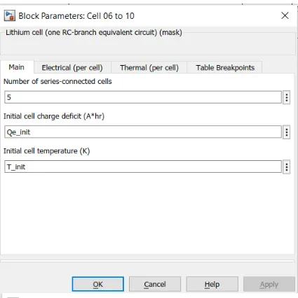
no of cells connected in series =5
initial temperature = 299.1k

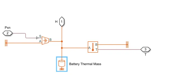
Thermal model:

thermal reference:

the thermal reference block represents a point with an absolute zero temperature, concerning which all the temperatures in the system are determined.

Controlled heat flow rate source:

the controlled heat flow rate source block represnets an ideal source of thermal energy that is powerful enough to maintain specified hear flow at its outlet regardless of the temperature difference across the source.
Connections A and B are thermal conserving ports corresponding to the source inlet and outlet, respectively. Port S is a physical signal port, through which the contol signal that drives the source is applied.
the heat flow through the source is directly proportional to the signal at the control port S.
the block positive direction is form port A to port B.
This means that positive signal at port S generates heat flow in the direction from A to B.

Thermal Mass:

the thermal mass block represents a thermal mass which reflects the ability of a material or a combination of materials to store internal energy.
the property is characterized by the mass of the material and its specific heat.
the thermal mass is described with the following equation.
Q=c.m*dT/dt
Temperature sensor:

the temperature sensor block represents and ideal temperature sensor,a device that determines the temperature differential measured between two points without drawing any heat.
connections A and B are thermal conserving ports that connect to the two points where the tenmperature is being monitored.
Port T ius a physical signal port A to port B.
The measured temperature is determined as T=TA-TB.
Temperature source:

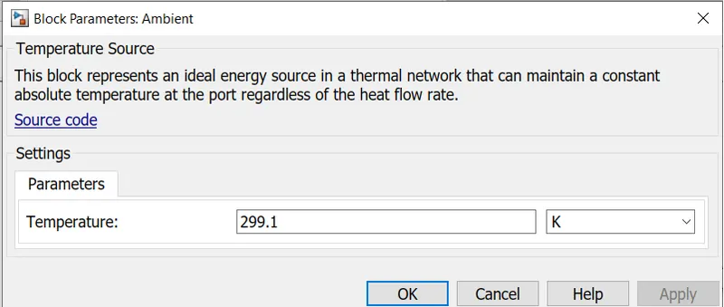
the temperature source block represents an ideal source of thermal energy that is powerful enough to maintain a specified temperature at its outlet regardless of the heat flow consumed by the system.
the source generates constant absolute temperature, defined by the temperature paramater value.
here i used ambient block and set the temperature for 299.1K ot 25.95C.

conductive heat transfer:

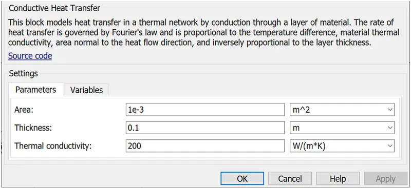
The conductive heat transfer block represents a heat transfer by conduction between two layers of the same material.
The transfer is govered by the fourier law and is described with the following equation:
Q=k.AD(TA-TB)

convective heat transfer:

the convective heat transfer block represents a heat transfer by convection between two bodies using fluid motion.
the transger is govered by the newton law of cooling and is described with the following equation.
Q=k.A.(TA-TB).

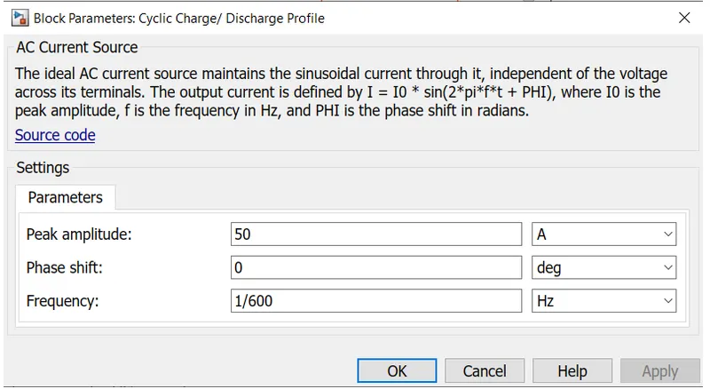
AC Current source:

the AC current source block represents an ideal current source that maintains the sinusoidal current throguh it, independent of the voltage across its terminals
the output current is defined by the following equation:

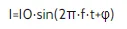
The peak amplitude is set to 50A for a cyclic charge and discharge. A basic parameter of AC source.

Electrical sensors:

the current sensor block represents an ideal current sensor, a device that converts current measured in aby electrical branch into a physical signal proportional to the current.
connections + and - are electrical conserving ports through which the sensors is inserted into the circuits.

Electrical Reference:

the Electrical reference block represents an electrical ground.
Electrical conserving ports of all the block that are directly connected to the ground must be connected to an electrical reference block.
A model with electrical elements must contain at least one electrical reference block.

Lithium cell 1RC Subsystem:

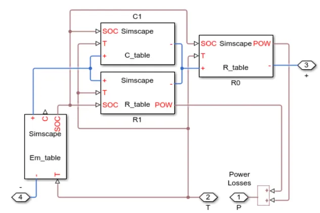
this block especially consists of the capacitor (C) value table which depends upon an external physical signal input SOC and T.
it is assumed that the capacitor value is varying with the time and hence the equation i=C*dV/dt holds.
|Resistance value (R) table depends on external physical signal inputs SOC and T.
Voltage value (EM) implements the cell's main branch voltage source and determines values for capacity (c) and state of charge (SOC).
The defining the equation depends upon cell temperature T.

SOC Calculation:

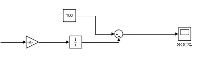
for SOC calculation here lets use gain block intergrator and sum block sum with PS Simulink Converter.

SIMULATION OF THE THERMAL EFFECTS, LIFE CYCLE PERFORMANCE AT VARIOUS TEMPERATURES, CHARGE AND DISCHARGE RATES:

• 10 lithium ion battery cells are connected in with the combination of three packs the first consistent 4 cells in series and the second pack consist of 1 cell which set to design as fault for study purpose to observe temperature changes within battery pack and the 3rd pack contains 5 cells in series.
• the heat transfer is observed between the packs by conductio and convection block which are modes of heat transfer.
• T susbsystem is attached in between every pack to plot the temperature graph of the cell of that particular battery pack.
• also external ambient temperature is attached and also thermal sensor is attached to the same to indicate the values in the display.
• also we added a current sensor in between the battery pack and AC current source to observe the cyclic charge and discharge rate graph.
• also we added a current sensor in between the battery pack and AC current source to calculate the SOC of the battery.
• the cell temperature and SOC graphs are plotted in scope while indicating the temperature of cell no 4, cell no 5 and cell no 10.
• all the other results are located in the simcape result menu.

for the study, we have some observation where we getting results for different cell temperature.
let us perform 3 tests with different temperates in each battery cells.

TEST 1:

let us set the ambient temperature as 299.1k.
cell temperature for 1 to 4 = 299.1 k
Cell temperature for 5 = 299.1 k,
Cell temperature for 6 to 10 = 299.1 K

Cell temperature for TEST 1 result:

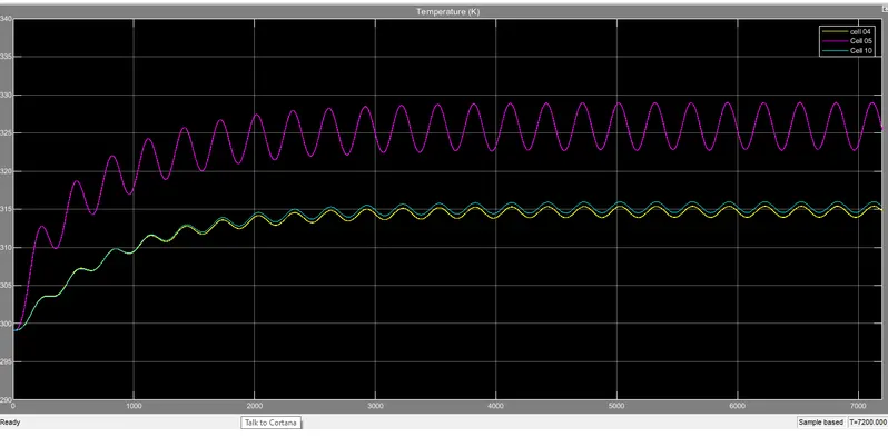
all the three cell having the same temperature at the start which is at 299.1 k. but in the begining few seconds of simulation cell no 5 oscillates with more than cell 4 and other beacuse its design with fault and ranging to higher temp than cell 4 and 10. after a time period of around 1300 sec both the cells getting are unfollwoing the temperature line whichw as following the same temperature rate, cell no 4 and 10 having approximately 315c(cell 4 having quite less temp then cell 10 because of no of the cell are differrent) k at the end of the simulation and the cell no 5 achieving the higher temperature of around 328 k.

SOC For TEST 1 Result:

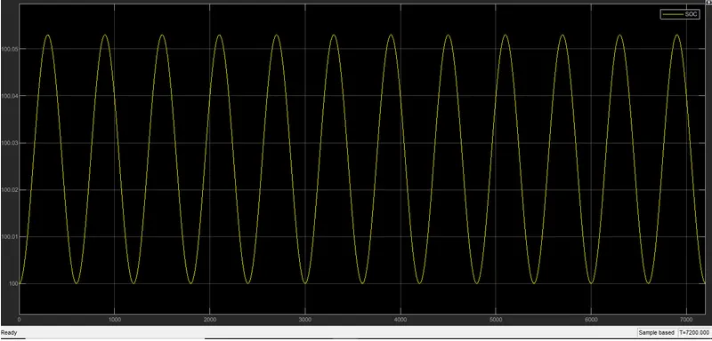
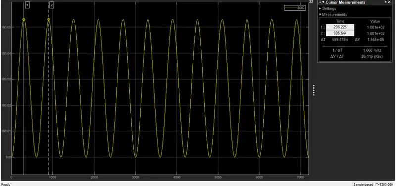
the SOC graph following the sinusoidal waveform structure and fluctuating after 297 seconds and this wave form is achieving the value of more than 100 % of SOC.

conduction:
conduction is basically heat flow rate(A) and temperature differenece with respect to time.

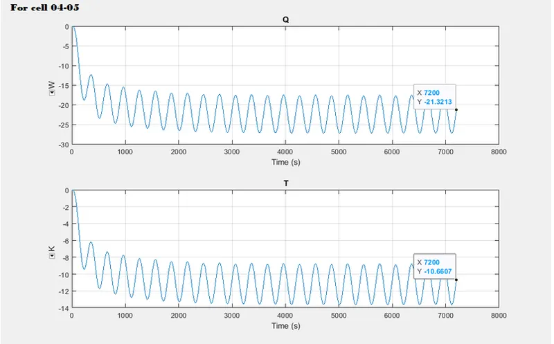
cell no 04-05 and having a high amplitue of waveforms(for heat flow and temperature difference) which are oscillating at a pretty high rate which is starting from zero and dropping into the negative zone at the end of simulation.
The heat transfer coefficient is -21.32 W/(m^2).k
thermal conductivity-10.66 W.m k

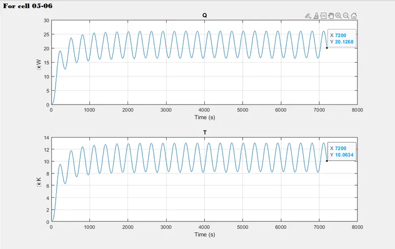
for cell 05 to 06 both the waveforms oscillating at a high rate but in a postive sone which are increasing initially and maintaining a certain range.
the heat transfer coefficinet is 20.12 W/(m^2).k
thermal conductivity 10.06 W/m.k

convection:
convection is the process of heat tranfer by the bulk movement of molecules within fluids such as gases and liquids.

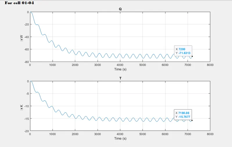
for cell no 1 to 4 the oscillations are pretty low and droppinf into the negative zone at the end of the simulation.
the final values for
the heat transfer coefficient is -71.63 W/(m^2)k
thermal conductivity -15.76 W/m k

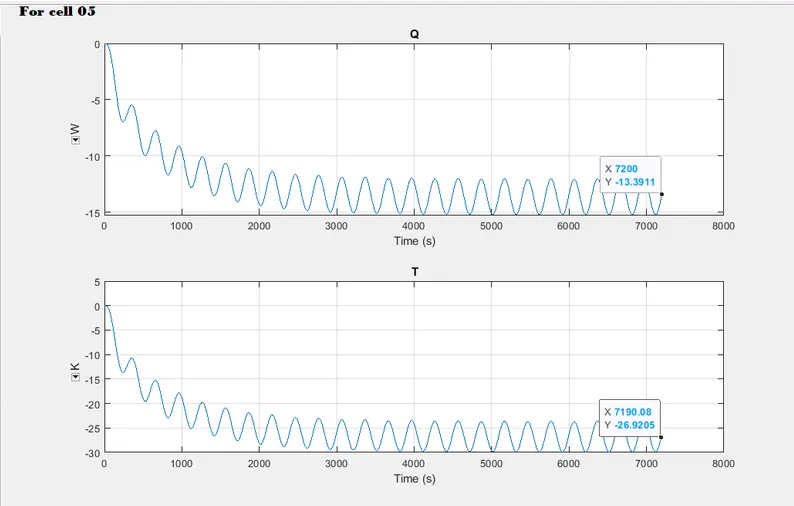
for cell no 5 they are staring from 0 and falling into the negative zone the oscillation having high amplitude because of the faulty cell at the end of the simulation.
the heat transfer coefficient is -13.39 W/(m^2).k
thermal conductivity -26.92 W/m.k

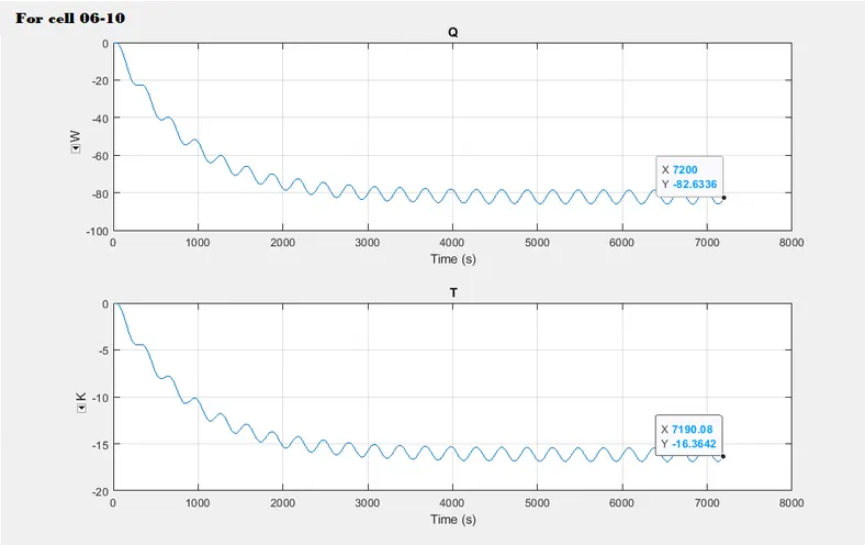
for cell 06 to 10 the falling zero to the negative zone the oscillation are less at the end of the simulation.
the heat transfer coefficient is -82.63 W/(m^2).k
thermal conductivity -16.36 W/m K.

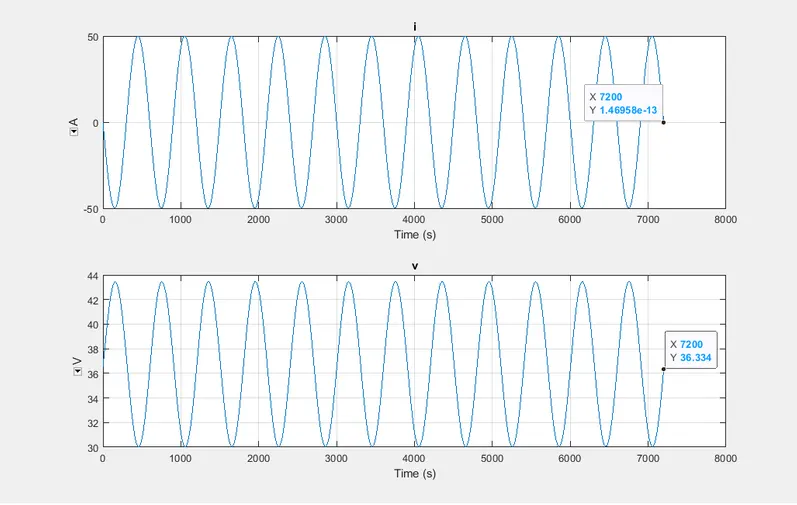
in the charge and discharge rate graph the voltage and current oscillating form pretty highly where current is ranging from -50 to 50 A and voltage is ranging from 30 to 43 volts.
the final value at the end of the simulation for
I (current) = 1.495e-13 A.
V (Voltage) = 36.334 Volt

TEST 2:
for the test 2 we take the ambient temperaure (k) = 299.1, cell temperature (k) (01-04) = 310.
Cell temperature (k) (05) = 299.1
cell temperature (k) (06 -10) = 310.

Cell Temperature:

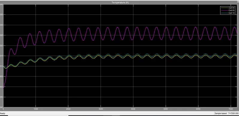
here the cell 04 and cell 10 starting from a temp of 310 k at the start of simulation and cell no 5 from 299.1k with higher oscillation as compared ot the other cells beacuse of faulty design at the end of the simulation, the cells 4 and 10 aving the final temp of nearby 315 k and cell no 5 achieving the temperature of 328 k.

SOC:

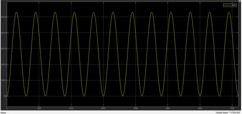
Conduction:

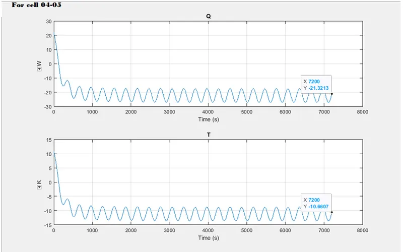
the heat flow rate plot srates form 20 and falls into the negative zone and the temperature difference plot starts from 10 and falls into the negative zone and oscillate at the end of the simulation the final value for,
the heat transfer coefficient is -21.32 W/(m^2).k
thermal conductivity -10.66 W/mk

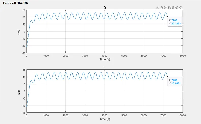
for cell no 5 to 6 the plot initiate form the negative zone and at the end settle down in the positive zone where the final values for.
the heat transfer coefficient is 20.12 W/(m^2).k
thermal conductivity 10.06 w/m k.

Convection:

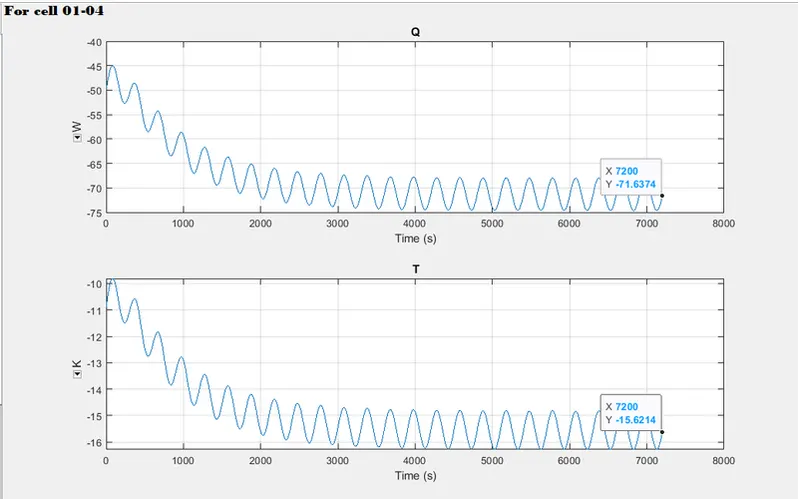
for cell no 1 to 4 the plot remains in the negative zone throughout the simulation with pretty low oscillation with falling nature and the final values at the end of the simulation are,
the heat transfer coefficient is -71.63 W/(m^2).k
thermal conductivity -15.62 W/m k

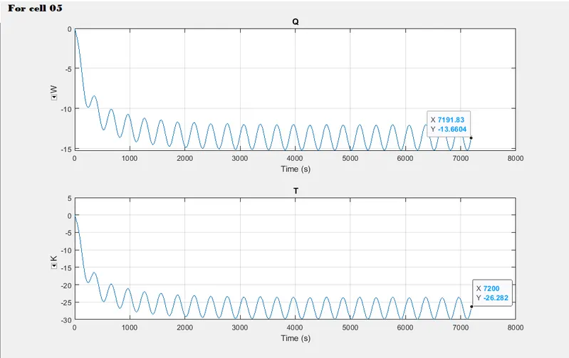
for cell no 5 the initial values are 0 and falling into the negative side with high oscillation because of the fault and the final values are,
the heat transfer coefficient is -13.66 W/(m^2) k.
thermal conductivity -26.28 W/m k.

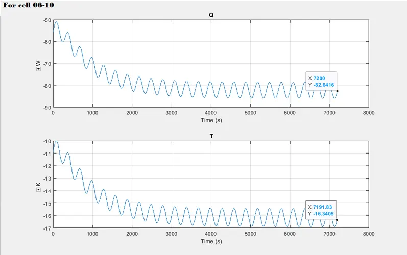
for cell 6 to 10 the plot remains on the negative side, and falling at the end of the simulation the final values are.
the heat transfer coefficient is -82.64 W/(m^2) k.
thermal conductivity -16.36 W/mk.

Charge and Discharge profile:

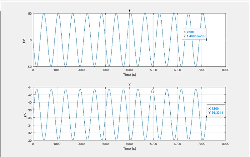
charge and discharge rate profile the plot for current is ranging in between -50 to 50A and voltage 30 to 43 volt and the final values for,
I (Current) = 1.4695e-13A
V (Volt) = 36.33 V.

TEST 3:
now lets run the 3rd test ambient temperature (k) = 299.1,
Cell temperature (k) (01-04)= 310,
cell temperature (k) (05) = 320,
cell temperature (k) (06-10) = 330.

Cell temperature:

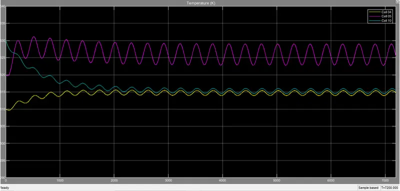
the initial temperature for cell 04 is 310 K, cell 5 is 320 k and cell 10 is 330 k, but after some point, cell no 04 and cell not 10 started following the same temperature rate, and cell no 5 starts oscillating with high value because of fault.
the final value for cell 04 and 10 is around 316 k and from cell no 5 is 328 k bacuse of its fault design.

SOC:

conduction:

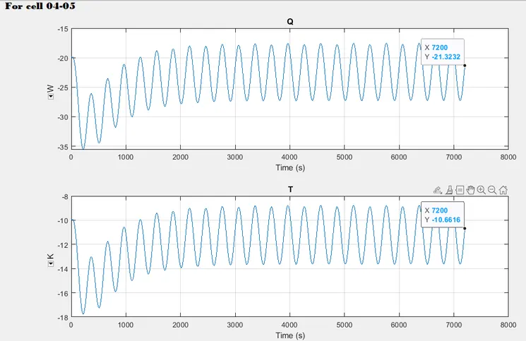
for cell 4 to 5 the plot starts from the negative side and drops and then again increases and maintians throughout the simulation negative zone. The final values at the end of the simulations are,
the heat transfer coefficient is -21.32 W/ (m^2) k,
thermal conductivity -10.66 W/m k.

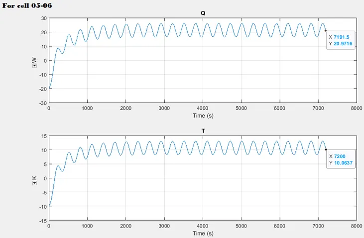
for cell no 5 to 6 both the plot starts form the negative side and then entered into the positive side and the final value at the end of the simulation are,
the heat trasnfer coefficient is 20/97 W/(m^2) k,
thermal conductivity 10.06 W/m k.

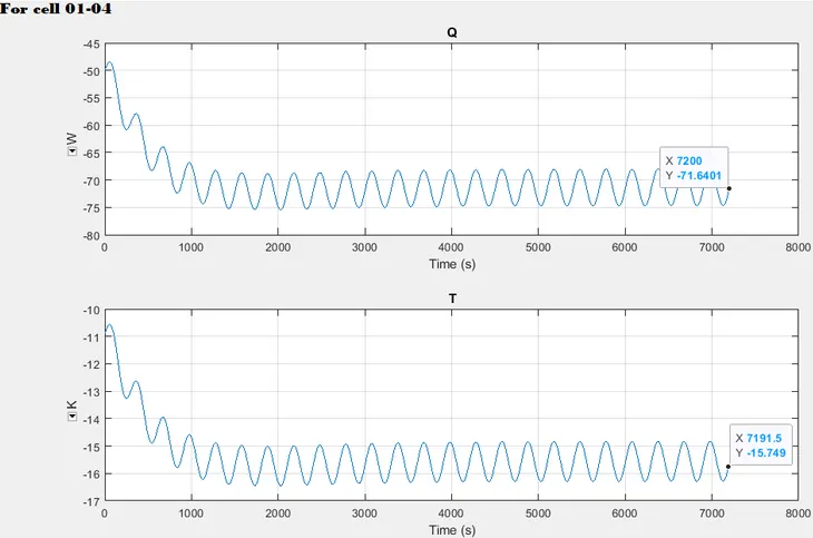
for cell no 01 to 04 the final values at the end of the simulation are,
the heat transfer coefficient is -71.64 W/(m^2) k.
thermal conductivity -15.75 W/mk.

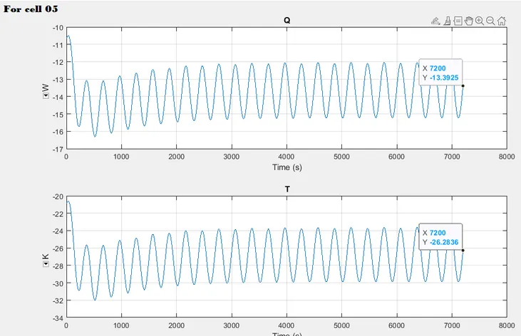
for cell 5 the final value at the end of the simulations are,
the heat transfer coefficient is -13.39 W/(m^2) k.
thermal conductivity -26.28 W/m k.

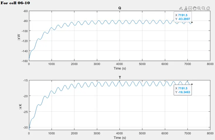
for cell no 6 to 10 the final values at the end of the simulation are,
the heat transfer coefficient is -83.30 W/(m^2) k,
thermal conductivity -16.34 W/ m k.

Charge and Discharge Profile:

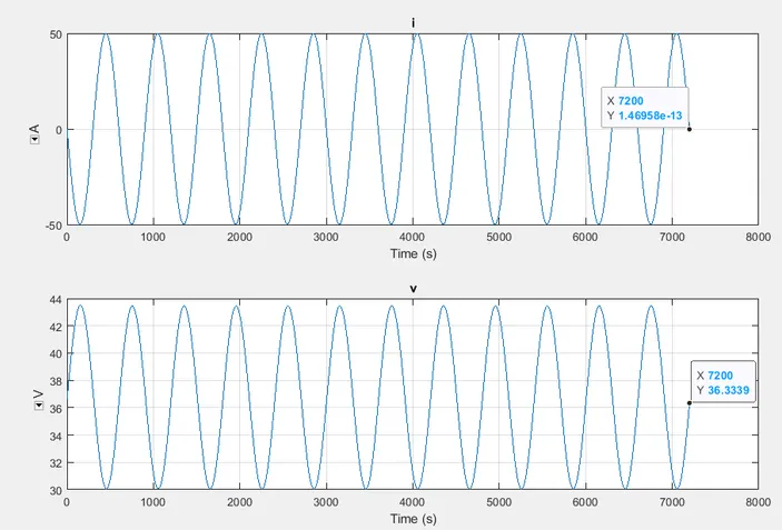
charge and discharge rate profile the plot for current is ranging between -50A to 50A and the voltage between 30V to43 V and the final values for,
I (Current) = 1.4695e-13A,
V (Volt) = 36.33 V.

CONCLUSIONS:

• as the difference in temperature we can observe the changes in the heat flow rate by conduction and convection.
• there are slight changes in cyclic charge and discharge as I fixed peak amplitude at 50A.
• SOC for all the temperature remain the same so there is no difference in SOC Graphs.
• Cell no 5 had higher oscillation and we an observe that in every graph because we design that cell for fault.

RESULT:

Thus the MATLAB simulink model for a for a 10 cell series lithium ion battery is modellled successfully and the simulaion of the thermal effects and comparision of life cycle performance at various temperatures, charge & discharge rates are completed and the output is verified.