Project 2 - Speed Control of a Direct Current (DC) motor

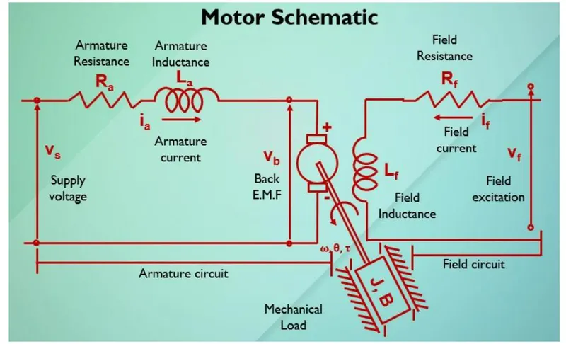
In this project, a Simulink model for the DC motor will be first developed per the schematic shown in Figure 1.

Use the Proportional, Integral, and Derivative (PID) control design knowledge gained in the training to design, develop and test a controller to maintain a desired speed for the motor.

Key Highlights:

• Mathematical modeling from the first principles
• Modeling an Electrical Engineering system
• Simulink based modeling
• Control law design and test
• Stability of a dynamic system

Deliverables:

• Matlab script to define modeling and control design parameters
• Simulink model to simulate and verify the design

Project

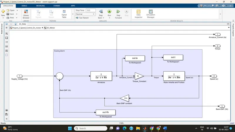
Simulink model without PID

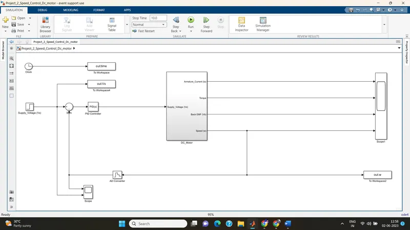
With PID control

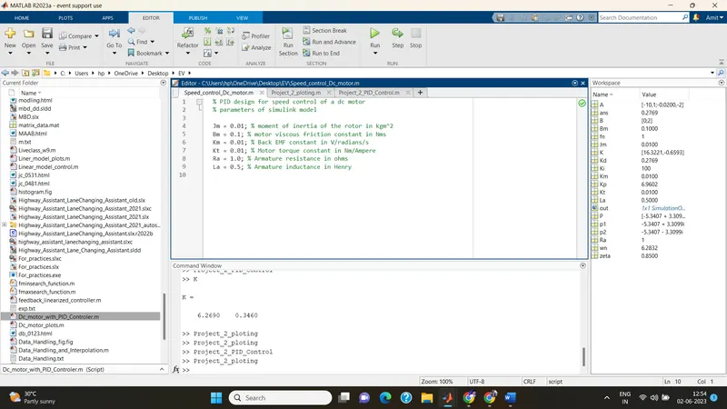
% PID design for speed control of a dc motor

% parameters of simulink model

Jm = 0.01; % moment of inertia of the rotor in kgm^2

Bm = 0.1; % motor viscous friction constant in Nms

Km = 0.01; % Back EMF constant in V/radians/s

Kt = 0.01; % Motor torque constant in Nm/Ampere

Ra = 1.0; % Armature resistance in ohms

La = 0.5; % Armature inductance in Henry

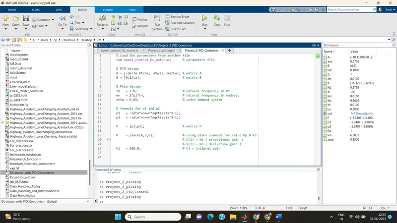
% Load the parameters from another file

run Speed_control_Dc_motor.m; % parameters file

% PID design

A = [-Bm/Jm Kt/Jm; -Km/La -Ra/La]; % matrix A

B = [0;1/La]; % matrix B

% Pole design

fn = 1.0; % natural frequency in Hz

wn = 2*pi*fn; % natural frequency in rad/sec

zeta = 0.85; % under damped system

% formula for p1 and p2

p1 = -zeta*wn+wn*sqrt(zeta^2-1);

p2 = -zeta*wn-wn*sqrt(zeta^2-1);

P = [p1;p2]; % matrix P

K = place(A,B,P); % using place command for value Kp & Kd

% K(1) = Kp ( propotional gain )

% K(2) = Kd ( derivative gain )

Ki = 100.0; % Ki = intigral gain

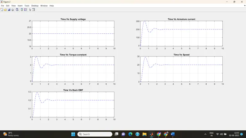
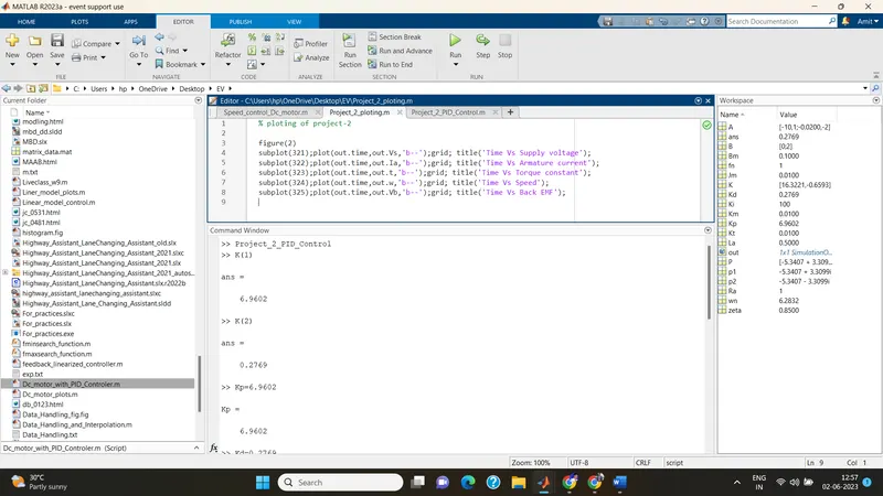
% ploting of project-2

figure(2)

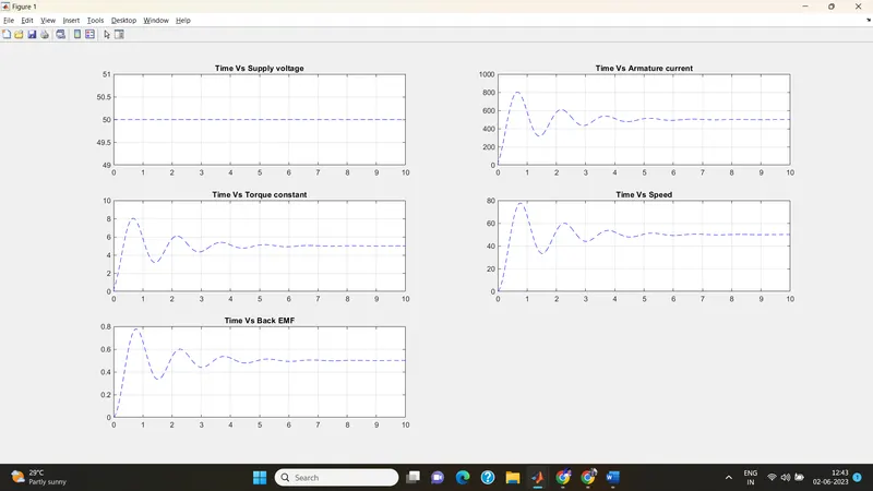
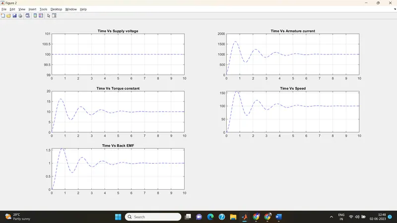
subplot(321);plot(out.time,out.Vs,'b--');grid; title('Time Vs Supply voltage');

subplot(322);plot(out.time,out.Ia,'b--');grid; title('Time Vs Armature current');

subplot(323);plot(out.time,out.t,'b--');grid; title('Time Vs Torque constant');

subplot(324);plot(out.time,out.w,'b--');grid; title('Time Vs Speed');

subplot(325);plot(out.time,out.Vb,'b--');grid; title('Time Vs Back EMF');

Without PID; Zeta 0.5; final value 230;

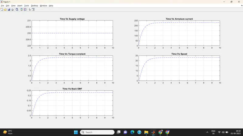
Final Value 50; zeta 0.999;

Final value 100; zeta 1.01 over damped system;

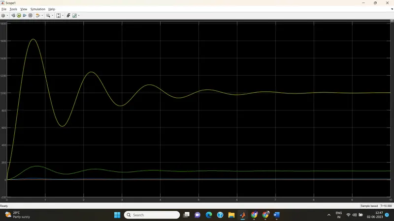
Final value 20; zeta 0.85;